Insurance Mathematics
💰 Why This Matters
Insurance mathematics reveal that frequency-severity modeling captures the dual nature of risk (how often losses occur and how severe they are), with heavy-tailed distributions like Pareto essential for modeling catastrophic events where traditional Gaussian assumptions fail to capture the true magnitude of the downside. The layer pricing framework shows why excess-of-loss structures dominate: they efficiently separate attritional losses (predictable, retained) from severity losses (volatile, transferred), optimizing the premium-to-protection tradeoff. Retention optimization through the ergodic lens demonstrates that optimal retention increases with wealth in absolute terms but decreases as a percentage of wealth; i.e., wealthier entities should retain more risk but proportionally less. The compound distribution mathematics proves that aggregate losses have fundamentally different properties than individual claims, explaining why reinsurers price differently than primary insurers. Claims development triangles and chain ladder methods quantify the time value of uncertainty, showing why early reserving decisions compound into material impacts. This framework transforms insurance from a cost center to a growth enabler by quantifying exactly how volatility reduction through strategic risk transfer enhances long-term compound returns, the mathematical foundation for why insurance creates value beyond simple loss indemnification.
Table of Contents

Frequency-Severity Models
Classical Framework
Insurance losses are modeled as a two-stage process:
Frequency: Number of claims in a period
Severity: Size of each claim
Total loss:
\(N\) = Number of claims (random)
\(X_i\) = Size of \(i\)-th claim (random)
Frequency Distributions
Poisson Distribution
Most common for claim counts:
Properties:
Mean = Variance = \(\lambda\)
Memoryless inter-arrival times
Suitable for homogeneous risks
Note: in practice, Over-Dispersed Poisson (ODP), where Variance exceeds the Mean, is preferred because claim estimation introduces uncertainty. For simplicity, we start the implementation with a regular Poisson model.
Negative Binomial
For overdispersed counts (variance > mean) and correlated claims:
Properties:
Mean = \(r(1-p)/p\)
Variance = \(r(1-p)/p^2\) > Mean
Captures heterogeneity via mixing
Zero-Inflated Models
When many policies have no claims:
Severity Distributions
Log-Normal
For moderate to large claims:
Properties:
Right-skewed
Multiplicative effects
No upper bound
Pareto
For extreme losses (heavy-tailed):
Properties:
Power-law tail
Infinite variance if \(\alpha \leq 2\)
Scale-invariant
Generalized Pareto (GPD)
For excess losses above threshold:
\(\xi\) = Shape parameter (tail index)
\(\sigma\) = Scale parameter
Implementation Example
import numpy as np
from scipy import stats
import matplotlib.pyplot as plt


class FrequencySeverityModel:
    """Model insurance losses using frequency-severity approach."""

    def __init__(self, freq_dist, sev_dist):
        self.freq_dist = freq_dist
        self.sev_dist = sev_dist

    def simulate_annual_loss(self, n_sims=10_000):
        """Simulate total annual losses."""
        total_losses = []

        for _ in range(n_sims):
            # Number of claims
            n_claims = self.freq_dist.rvs()

            if n_claims == 0:
                total_losses.append(0)
            else:
                # Individual claim amounts
                claims = self.sev_dist.rvs(size=n_claims)
                total_losses.append(np.sum(claims))

        return np.array(total_losses)

    def calculate_statistics(self, losses):
        """Calculate key statistics."""
        return {
            'mean': np.mean(losses),
            'std': np.std(losses),
            'median': np.median(losses),
            'p95': np.percentile(losses, 95),
            'p99': np.percentile(losses, 99),
            'p99.5': np.percentile(losses, 99.5),
            'max': np.max(losses),
            'prob_zero': np.mean(losses == 0)
        }

    def plot_distribution(self, losses):
        """Visualize loss distribution."""
        fig, axes = plt.subplots(2, 2, figsize=(12, 10))

        # Histogram
        axes[0, 0].hist(losses[losses > 0], bins=50,
                        edgecolor='black', alpha=0.7)
        axes[0, 0].set_xlabel('Loss Amount')
        axes[0, 0].set_ylabel('Frequency')
        axes[0, 0].set_title('Loss Distribution (excluding zeros)')

        # Log-log plot for tail
        sorted_losses = np.sort(losses[losses > 0])
        exceedance_prob = np.arange(len(sorted_losses), 0, -1) / len(losses)
        axes[0, 1].loglog(sorted_losses, exceedance_prob)
        axes[0, 1].set_xlabel('Loss Amount (log scale)')
        axes[0, 1].set_ylabel('Exceedance Probability (log scale)')
        axes[0, 1].set_title('Tail Behavior')

        # Recreate Q-Q plot manually to control colors: data points in default blue, fit line in orange
        (osm, osr), (slope, intercept, r) = stats.probplot(
            np.log(losses[losses > 0]), dist="norm", fit=True)
        axes[1, 0].plot(osm, osr, marker='.', linestyle='none',
                        markersize=4, color='C0', alpha=0.8)
        axes[1, 0].plot(osm, slope * np.asarray(osm) + intercept,
                        color='orange', linestyle='--', linewidth=1.5)

        # Empirical CDF
        axes[1, 1].plot(sorted_losses, np.arange(
            1, len(sorted_losses) + 1) / len(sorted_losses))
        axes[1, 1].set_xlabel('Loss Amount')
        axes[1, 1].set_ylabel('Cumulative Probability')
        axes[1, 1].set_title('Empirical CDF')
        axes[1, 1].grid(True, alpha=0.3)

        plt.tight_layout()
        return fig


# Example: Commercial property insurance
freq_dist = stats.poisson(mu=3)  # 3 claims per year on average
sev_dist = stats.lognorm(s=2, scale=50_000)  # Log-normal severity

model = FrequencySeverityModel(freq_dist, sev_dist)
losses = model.simulate_annual_loss(n_sims=10_000)
statistics = model.calculate_statistics(losses)

model.plot_distribution(losses)

print("Annual Loss Statistics:")
for key, value in statistics.items():
    if key == 'prob_zero':
        print(f"{key}: {value:.1%}")
    else:
        print(f"{key}: ${value:,.0f}")
Sample Output
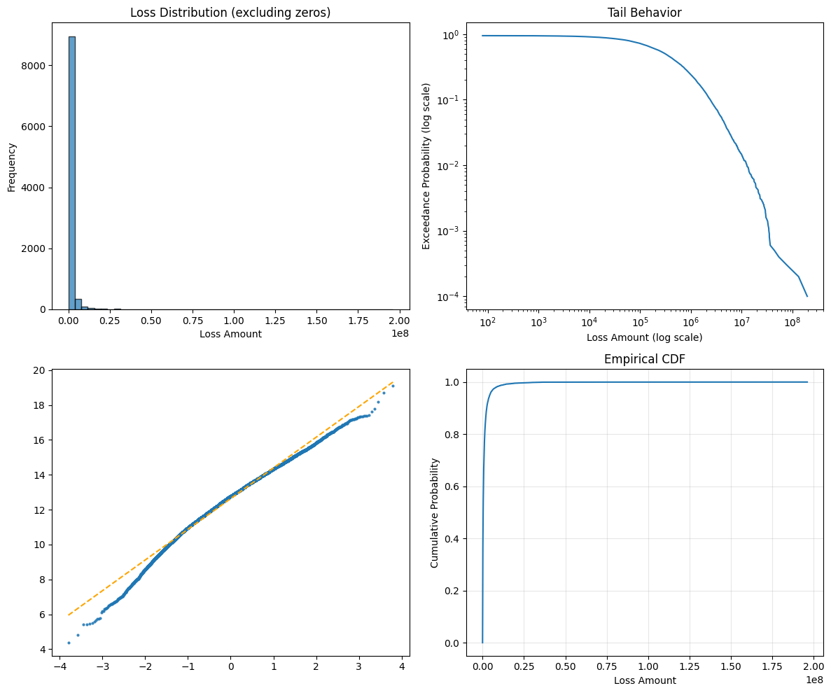
Annual Loss Statistics:
mean: $1,089,751
std: $3,579,880
median: $318,641
p95: $4,191,252
p99: $12,699,935
p99.5: $18,849,964
max: $196,094,596
prob_zero: 5.0%
Compound Distributions
Definition
The compound distribution of total losses \(S = \sum_{i=1}^N X_i\) has:
Characteristic function:
where \(G_N\) is the probability generating function of \(N\).
Compound Poisson
When frequency \(N \sim \text{Poisson}(\lambda)\) and severities \(X_i\) are i.i.d.:
Mean: \(E[S] = \lambda \cdot E[X]\) Variance: \(\text{Var}(S) = \lambda \cdot E[X^2]\) Skewness: \(\text{Skew}(S) = \frac{E[X^3]}{\lambda^{1/2} \cdot E[X^2]^{3/2}}\)
Panjer Recursion
For discrete severities, recursive approximation of \(S\) is given by:
where:
\(p_k = P(S = k)\)
\(f_j = P(X = j)\)
\((a, b)\) depend on frequency distribution
Fast Fourier Transform Method
FFT provides a computationally efficient approach for determining the aggregate loss distribution for a given frequency-severity model. The method exploits the relationship between the characteristic functions and probability generating functions.
For continuous distributions:
import numpy as np
from scipy import stats
import matplotlib.pyplot as plt


def compound_distribution_fft(freq_params, sev_params, x_max=1e8, n_points=2**16):
    """Calculate compound distribution using FFT - CORRECTED."""

    dx = x_max / n_points
    x = np.arange(n_points) * dx

    # Discretize severity distribution WITHOUT normalization
    sev_pmf = stats.lognorm.pdf(x[1:], s=sev_params["s"], scale=sev_params["scale"]) * dx

    # Prepend zero for x[0] since individual claims can't be zero
    sev_pmf = np.concatenate([[0], sev_pmf])

    # Check how much probability mass we captured (should be close to 1)
    captured_mass = sev_pmf.sum()
    print(f"Captured severity mass: {captured_mass:.6f}")

    # DON'T normalize - use the natural discretization
    # The small missing mass in the tail is acceptable

    # FFT operations
    sev_cf = np.fft.fft(sev_pmf)
    lambda_param = freq_params["lambda"]
    compound_cf = np.exp(lambda_param * (sev_cf - 1))
    compound_pmf = np.real(np.fft.ifft(compound_cf))

    # The compound_pmf now contains:
    # - At index 0: P(S = 0) (point mass)
    # - At other indices: probability masses for discretized positive values

    prob_zero = compound_pmf[0]

    # Convert to density (but keep point mass separate)
    pdf = compound_pmf / dx
    pdf[0] = 0  # Remove point mass from density

    return x, pdf, prob_zero

# Calculate FFT solution
freq_params={"lambda": 3}
sev_params={"s": 2, "scale": 50_000}
x, pdf, prob_zero = compound_distribution_fft(freq_params=freq_params, sev_params=sev_params)

# Simulate
n_sims = 100_000
freq = stats.poisson(mu=3)
sev = stats.lognorm(s=2, scale=50_000)

sim_losses = np.zeros(n_sims)
for i in range(n_sims):
    n_claims = freq.rvs()
    if n_claims > 0:
        sim_losses[i] = sev.rvs(size=n_claims).sum()

plt.figure(figsize=(10, 6))

# Plot with adjusted bins
x_plot_max = x[999]
bin_edges = np.concatenate([[0, 1], np.linspace(1, x_plot_max, 199)])
plt.hist(sim_losses, bins=bin_edges, density=True,
         alpha=0.45, color='C1', zorder=1, label='Simulated (adjusted bins)')

# Plot continuous part
plt.semilogy(x[1:1000], pdf[1:1000], label='FFT-based Density', linewidth=2)

# Mark the point mass
plt.scatter([0], [pdf[1]], color='red', s=100, zorder=5,
            label=f'Point mass: {prob_zero:.3f}')

plt.xlabel("Total Annual Loss")
plt.ylabel("Probability Density (log scale)")
plt.title("Compound Poisson-Lognormal Distribution")
plt.grid(True, alpha=0.3)
plt.legend(loc='best')
plt.show()

# Better validation: Compare key statistics
sim_mean = np.mean(sim_losses)
sim_std = np.std(sim_losses)

# Theoretical values
theory_mean = freq_params["lambda"] * stats.lognorm.mean(s=sev_params["s"], scale=sev_params["scale"])
theory_var = (freq_params["lambda"] *
              stats.lognorm.var(s=sev_params["s"], scale=sev_params["scale"]) +
              freq_params["lambda"] *
              stats.lognorm.mean(s=sev_params["s"], scale=sev_params["scale"])**2)
theory_std = np.sqrt(theory_var)

print(f"\nValidation Statistics:")
print(f"Mean - Simulated: {sim_mean:,.0f}, Theoretical: {theory_mean:,.0f}")
print(f"Std Dev - Simulated: {sim_std:,.0f}, Theoretical: {theory_std:,.0f}")
print(f"P(Loss = 0) - Simulated: {np.mean(sim_losses == 0):.4f}, Theoretical: {prob_zero:.4f}")
Sample Output
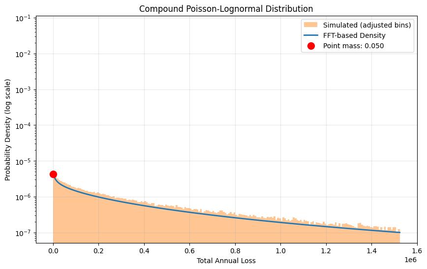
Validation Statistics:
Mean - Simulated: 1,109,983, Theoretical: 1,108,358
Std Dev - Simulated: 4,216,943, Theoretical: 4,728,338
P(Loss = 0) - Simulated: 0.0496, Theoretical: 0.0498
Layer Pricing Theory
Excess of Loss Layers Insurance coverage is structured in layers:
Primary: \(\$0\) to \(L_1\)
First Excess: \(L_1\) to \(L_2\)
Second Excess: \(L_2\) to \(L_3\), etc.
Layer Loss Calculation
For layer\([a, b]\), the loss is:
Expected layer loss:
Increased Limits Factors (ILFs)
Ratio of expected loss at different limits:
where \(L_0\) is the base limit.
Exposure Curves
Proportion of loss in layer:
where \(M\) is the maximum possible loss.
Layer Pricing Example
For an exploration of Insurance Layers, see this Jupyter Notebook on Insurance Layer Optimization.
Retention Optimization
Objective Function
Maximize utility or growth:
\(R\) = Retention level
\(P(R)\) = Premium function
\(L\) = Random loss
\(W\) = Initial wealth
This function balances lower premium \(P(R)\) vs risk exposure \((L \wedge R)\).
First-Order Condition
For differentiable utility: $\( P'(R) = E[U'(W - P(R) - (L \wedge R)) \cdot \mathbf{1}_{L > R}] \)$
Ergodic Optimization
Maximize time-average growth:
Constraints
Budget constraint:\(P(R) \leq B\)
Ruin constraint:\(P(\text{ruin}) \leq \alpha\)
Regulatory minimum: \(R \geq R_{\text{min}}\)
Ergodic Optimization Example
import numpy as np
import matplotlib.pyplot as plt
from scipy import stats, optimize
from scipy.integrate import quad
import warnings
warnings.filterwarnings('ignore')
# ============================================
# 1. CORRECTED PREMIUM AND OBJECTIVE FUNCTIONS
# ============================================
def premium_function(R, expected_loss, loading=0.3, expense_ratio=0.05):
"""
Premium function for retention R.
Premium decreases as retention increases (you keep more risk).
"""
# Create loss distribution (lognormal with CV = 0.5)
loss_dist = stats.lognorm(s=0.5, scale=expected_loss)
# Calculate E[max(L - R, 0)] using the lognormal properties
# More efficient calculation using CDF
def excess_loss(R):
if R <= 0:
return expected_loss
# For lognormal, we can use the partial expectation formula
mu = np.log(expected_loss) - 0.5 * 0.5**2
sigma = 0.5
# Partial expectation E[L * 1{L>R}]
z = (np.log(R) - mu - sigma**2) / sigma
partial_exp = expected_loss * np.exp(0.5 * sigma**2) * (1 - stats.norm.cdf(z))
# E[max(L-R, 0)] = E[L * 1{L>R}] - R * P(L>R)
prob_exceed = 1 - loss_dist.cdf(R)
expected_excess = partial_exp - R * prob_exceed
return expected_excess
# Expected excess loss
expected_excess = excess_loss(R)
# Premium with loading and expenses
premium = (1 + loading) * expected_excess + expense_ratio * expected_loss
return premium
def ergodic_objective(R, wealth, loss_dist, loading=0.3):
"""
Corrected ergodic objective: E[ln(W - P(R) - min(L, R))]
"""
# Calculate premium for this retention
premium = premium_function(R, loss_dist.mean(), loading)
# Check if we can afford this strategy
if premium >= wealth * 0.9: # Can't spend 90%+ of wealth on premium
return -np.inf
# More samples for better accuracy
np.random.seed(42)
n_samples = 50000
losses = loss_dist.rvs(n_samples)
# Calculate retained losses
retained_losses = np.minimum(losses, R)
# Final wealth for each scenario
final_wealth = wealth - premium - retained_losses
# Check for bankruptcy
if np.any(final_wealth <= 0):
# Calculate probability-weighted utility including bankruptcy scenarios
valid = final_wealth > 0
if not valid.any():
return -np.inf
# Penalize strategies that lead to bankruptcy
bankruptcy_penalty = -100 # Large negative utility for bankruptcy
utility = np.where(valid, np.log(final_wealth), bankruptcy_penalty)
return np.mean(utility)
# Expected log wealth (ergodic growth rate)
return np.mean(np.log(final_wealth))
def solve_ergodic_retention(wealth, expected_loss=100_000, loading=0.3, cv=0.5):
"""
Find optimal retention that maximizes ergodic growth rate.
Uses global optimization to avoid local minima.
"""
# Create loss distribution
loss_dist = stats.lognorm(s=cv, scale=expected_loss)
# Objective function (negative for minimization)
def neg_objective(R):
return -ergodic_objective(R, wealth, loss_dist, loading)
# Bounds: retention between small value and reasonable maximum
min_retention = expected_loss * 0.001 # Very small retention
max_retention = min(wealth * 0.3, expected_loss * 3) # Conservative upper bound
# Use global optimization to avoid local minima
from scipy.optimize import differential_evolution
result = differential_evolution(
neg_objective,
bounds=[(min_retention, max_retention)],
seed=42,
maxiter=100,
workers=1
)
optimal_retention = result.x[0]
optimal_growth_rate = -result.fun
return optimal_retention, optimal_growth_rate
# ============================================
# 2. IMPROVED DYNAMIC PROGRAMMING
# ============================================
def dp_ergodic_retention(wealth_grid, loss_dist, n_periods=10,
loading=0.3, discount=0.95):
"""
Improved DP using continuous optimization at each step instead of grid search
"""
n_wealth = len(wealth_grid)
# Store optimal retentions (continuous values, not grid indices)
optimal_retentions = np.zeros((n_periods, n_wealth))
V = np.zeros((n_periods + 1, n_wealth))
# Terminal value
V[-1, :] = np.log(np.maximum(wealth_grid, 1e-6))
# Backward induction with continuous optimization
for t in range(n_periods - 1, -1, -1):
for i, w in enumerate(wealth_grid):
# Define objective for this (t, w) pair
def objective(R):
# Calculate immediate payoff and continuation value
premium = premium_function(R, loss_dist.mean(), loading)
if premium > w * 0.3 or R > w * 0.5:
return -np.inf
# Sample losses
losses = loss_dist.rvs(2000)
retained = np.minimum(losses, R)
next_wealth = w - premium - retained
valid = next_wealth > 0
if not valid.any():
return -np.inf
current_util = np.mean(np.log(next_wealth[valid]))
if t < n_periods - 1:
# Interpolate continuation values
from scipy.interpolate import interp1d
value_func = interp1d(wealth_grid, V[t + 1, :],
kind='cubic', bounds_error=False,
fill_value='extrapolate')
continuation = discount * np.mean(value_func(next_wealth[valid]))
else:
continuation = 0
return current_util + continuation
# Continuous optimization instead of grid search
from scipy.optimize import minimize_scalar
# Smart bounds based on wealth level
R_min = max(1000, w * 0.001)
R_max = min(w * 0.3, loss_dist.mean() * 2)
result = minimize_scalar(
lambda R: -objective(R),
bounds=(R_min, R_max),
method='bounded'
)
optimal_retentions[t, i] = result.x
V[t, i] = -result.fun
return V, optimal_retentions
# ============================================
# 3. ANALYSIS WITH CORRECTIONS
# ============================================
# Set up parameters
expected_loss = 100_000
cv = 0.5
loading = 0.3
loss_dist = stats.lognorm(s=cv, scale=expected_loss)
# 1. Single-period analysis
print("Running single-period analysis...")
wealth_levels = np.linspace(500_000, 20_000_000, 20)
optimal_retentions = []
growth_rates = []
for wealth in wealth_levels:
R_opt, g_opt = solve_ergodic_retention(wealth, expected_loss, loading, cv)
optimal_retentions.append(R_opt)
growth_rates.append(g_opt)
print(f"Wealth ${wealth/1e6:.1f}M: Retention ${R_opt/1e3:.1f}K")
optimal_retentions = np.array(optimal_retentions)
growth_rates = np.array(growth_rates)
# 2. Multi-period DP with finer grids
print("\nRunning multi-period DP...")
wealth_grid_dp = np.linspace(500_000, 10_000_000, 15) # Fewer wealth points for speed
V, optimal_policy = dp_ergodic_retention(wealth_grid_dp, loss_dist,
n_periods=10, loading=loading,
discount=0.95)
# 3. Compare different loadings (CORRECTED EXPECTATION)
print("\nAnalyzing loading effects...")
loadings = [0.1, 0.3, 0.5, 0.7]
retention_by_loading = {}
for load in loadings:
print(f"Loading {load:.1%}...")
retentions = []
for wealth in wealth_levels:
R_opt, _ = solve_ergodic_retention(wealth, expected_loss, load, cv)
retentions.append(R_opt)
retention_by_loading[load] = np.array(retentions)
# ============================================
# 4. PLOTTING WITH CORRECTIONS
# ============================================
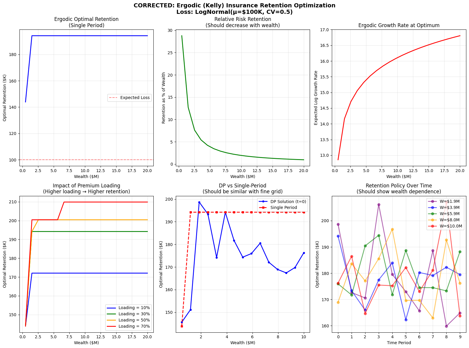
fig = plt.figure(figsize=(16, 12))
# Plot 1: Optimal retention vs wealth
ax1 = plt.subplot(2, 3, 1)
ax1.plot(wealth_levels/1e6, optimal_retentions/1e3, 'b-', linewidth=2)
ax1.set_xlabel('Wealth ($M)')
ax1.set_ylabel('Optimal Retention ($K)')
ax1.set_title('Ergodic Optimal Retention\n(Single Period)')
ax1.grid(True, alpha=0.3)
ax1.axhline(y=expected_loss/1e3, color='r', linestyle='--', alpha=0.5, label='Expected Loss')
ax1.legend()
# Plot 2: Retention as percentage of wealth
ax2 = plt.subplot(2, 3, 2)
retention_pct = (optimal_retentions / wealth_levels) * 100
ax2.plot(wealth_levels/1e6, retention_pct, 'g-', linewidth=2)
ax2.set_xlabel('Wealth ($M)')
ax2.set_ylabel('Retention as % of Wealth')
ax2.set_title('Relative Risk Retention\n(Should decrease with wealth)')
ax2.grid(True, alpha=0.3)
# Plot 3: Expected growth rate
ax3 = plt.subplot(2, 3, 3)
ax3.plot(wealth_levels/1e6, growth_rates, 'r-', linewidth=2)
ax3.set_xlabel('Wealth ($M)')
ax3.set_ylabel('Expected Log Growth Rate')
ax3.set_title('Ergodic Growth Rate at Optimum')
ax3.grid(True, alpha=0.3)
# Plot 4: Effect of loading (CORRECTED)
ax4 = plt.subplot(2, 3, 4)
colors = ['blue', 'green', 'orange', 'red']
for (load, retentions), color in zip(retention_by_loading.items(), colors):
ax4.plot(wealth_levels/1e6, retentions/1e3, linewidth=2,
label=f'Loading = {load:.0%}', color=color)
ax4.set_xlabel('Wealth ($M)')
ax4.set_ylabel('Optimal Retention ($K)')
ax4.set_title('Impact of Premium Loading\n(Higher loading → Higher retention)')
ax4.grid(True, alpha=0.3)
ax4.legend()
# Verify the relationship
wealth_test = 5_000_000
print(f"\nVerifying loading relationship at ${wealth_test/1e6}M wealth:")
for load in loadings:
idx = np.argmin(np.abs(wealth_levels - wealth_test))
ret = retention_by_loading[load][idx]
print(f" Loading {load:.0%}: Retention ${ret/1e3:.1f}K")
# Plot 5: Multi-period vs single-period (with finer grid)
ax5 = plt.subplot(2, 3, 5)
ax5.plot(wealth_grid_dp/1e6, optimal_policy[0, :]/1e3, 'b-', linewidth=2,
label='DP Solution (t=0)', marker='o', markersize=4)
# Compute single-period for comparison
sp_retentions = []
for w in wealth_grid_dp:
R_opt, _ = solve_ergodic_retention(w, expected_loss, loading, cv)
sp_retentions.append(R_opt)
ax5.plot(wealth_grid_dp/1e6, np.array(sp_retentions)/1e3, 'r--',
linewidth=2, label='Single Period', marker='s', markersize=4)
ax5.set_xlabel('Wealth ($M)')
ax5.set_ylabel('Optimal Retention ($K)')
ax5.set_title('DP vs Single-Period\n(Should be similar with fine grid)')
ax5.grid(True, alpha=0.3)
ax5.legend()
# Plot 6: Retention over time (FIXED to show wealth dependence)
ax6 = plt.subplot(2, 3, 6)
time_periods = np.arange(optimal_policy.shape[0])
wealth_indices = [2, 5, 8, 11, 14] # More spread out indices
colors_time = ['purple', 'blue', 'green', 'orange', 'red']
for idx, color in zip(wealth_indices, colors_time):
if idx < len(wealth_grid_dp):
wealth_val = wealth_grid_dp[idx]
ax6.plot(time_periods, optimal_policy[:, idx]/1e3,
linewidth=2, label=f'W=${wealth_val/1e6:.1f}M',
marker='o', color=color, alpha=0.6)
ax6.set_xlabel('Time Period')
ax6.set_ylabel('Optimal Retention ($K)')
ax6.set_title('Retention Policy Over Time\n(Should show wealth dependence)')
ax6.grid(True, alpha=0.3)
ax6.legend()
ax6.set_xticks(time_periods)
plt.suptitle('CORRECTED: Ergodic (Kelly) Insurance Retention Optimization\n' +
f'Loss: LogNormal(μ=${expected_loss/1e3:.0f}K, CV={cv})',
fontsize=14, fontweight='bold')
plt.tight_layout()
plt.show()
Sample Output
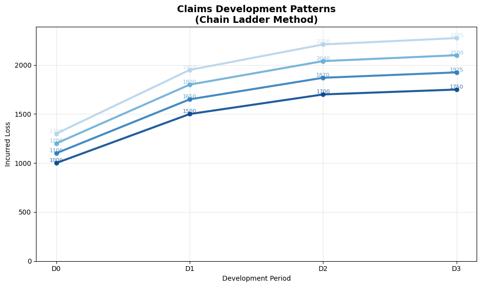
Claims Development
Development Triangles
Claims develop over time as they get reported and processed.
Here is an example of how actuaries organize development:
Poliy |
12 Months |
24 Months |
36 Months |
48 Months |
Ultimate |
|---|---|---|---|---|---|
2020 |
100 |
150 |
170 |
175 |
176 |
2021 |
110 |
165 |
187 |
? |
? |
2022 |
120 |
180 |
? |
? |
? |
2023 |
130 |
? |
? |
? |
? |
Vertically are batches of claims, usually by Policy Year, Accident Year, Report Year, or Calendar Year.
Going across are the same batches as they age over valuation dates.
Chain Ladder Method
Development factors:
The development factors are then judgmentally adjusted for reasonability and consistency with industry to arrive at \(f_j^*\)
Ultimate loss:
In practice, the triangles are finite, so typically there is a cutoff for available data, and a tail factor is applied judgmentally based on a separate study:
Chain Ladder Example
Continuing with the prior example, we compute the development factors:
Poliy |
12:24 |
24:36 |
36:48 |
48:Ultimate |
|---|---|---|---|---|
2020 |
1.5 |
1.13 |
1.03 |
1.01 |
2021 |
1.5 |
1.13 |
? |
? |
2022 |
1.5 |
? |
? |
? |
Since all the factors happen to agree for each age, we’ll select the factors without any adjustment, rounded as shown.
Age-to-Age Factors |
12:24 |
24:36 |
36:48 |
48:Ultimate |
|---|---|---|---|---|
Selected |
1.5 |
1.13 |
1.03 |
1.01 |
Age-to-Ultimate Factors |
12:Ult |
24:Ult |
36:Ult |
48:Ult |
|---|---|---|---|---|
Selected |
1.76 |
1.18 |
1.04 |
1.01 |
We can now fill the rightmost column of the triangle:
Poliy |
12 Months |
24 Months |
36 Months |
48 Months |
Ultimate |
|---|---|---|---|---|---|
2020 |
100 |
150 |
170 |
175 |
176 |
2021 |
110 |
165 |
187 |
? |
194 |
2022 |
120 |
180 |
? |
? |
212 |
2023 |
130 |
? |
? |
? |
229 |
These are ultimate claim estimates for each Policy Year, reliable under the following conditions:
Historical patterns of loss development are stable and consistent.
These historical patterns can be reliably projected into the future.
The book of business is neither growing nor shrinking rapidly.
Bornhuetter-Ferguson Method
Combines a prior estimate (typically Expected Claims Method) with actual incurred:
This assumes claims incurred to date for the period bear no predictability of future development.
Oftentimes, \((\text{\% Undeveloped})_k\) is estimated using Chain Ladder:
This holds since \(f_k^* = (\text{Proportional Future Ultimate}) = 1 + (\text{Proportional Future Development})\), so we have:
Either method can be performed on Incurred amounts or Paid amounts, with Paid typically giving more volatile estimates.
Implementation
class ClaimsDevelopment:
    """Model claims development patterns."""

    def __init__(self, triangle):
        self.triangle = np.array(triangle)
        self.n_years, self.n_dev = self.triangle.shape

    def chain_ladder(self):
        """Apply chain ladder method."""

        # Calculate development factors
        factors = []
        for j in range(self.n_dev - 1):
            numerator = np.nansum(self.triangle[:, j + 1])
            denominator = np.nansum(self.triangle[:self.n_years - j - 1, j])
            factors.append(numerator / denominator)

        # Apply factors to complete triangle
        completed = self.triangle.copy()

        for i in range(self.n_years):
            for j in range(self.n_years - i, self.n_dev):
                if np.isnan(completed[i, j]):
                    completed[i, j] = completed[i, j - 1] * factors[j - 1]

        return completed, factors

    def plot_development(self, completed):
        """Visualize development patterns."""

        # Use explicit figure and axis so we can return the local figure
        fig, ax = plt.subplots(figsize=(10, 6))

        # x coordinates for development periods
        x = np.arange(self.n_dev)

        # Color map for accident years (older darker, younger lighter)
        cmap = plt.cm.Blues
        colors = [cmap(0.9 - 0.6 * (i / max(1, self.n_years - 1))) for i in range(self.n_years)]

        # Plot development curve for each accident year and annotate
        for i in range(self.n_years):
            y = completed[i, :]
            ax.plot(x, y, color=colors[i], linewidth=3, marker='o', markersize=6,
                    zorder=3, alpha=0.9)
            for k, val in enumerate(y):
                if not np.isnan(val):
                    ax.text(k, val, f'{val:.0f}', fontsize=8, va='bottom', ha='center',
                            color=colors[i], alpha=0.8)

        # Set axes to development-period (x) vs incurred loss (y)
        ax.set_xlabel('Development Period')
        ax.set_ylabel('Incurred Loss')
        ax.set_xticks(x)
        ax.set_xticklabels([f'D{d}' for d in x])
        ax.set_ylim(0, np.nanmax(completed) * 1.05)
        ax.set_title('Claims Development Patterns\n(Chain Ladder Method)', fontsize=14, fontweight='bold')
        ax.grid(True, alpha=0.3)

        plt.tight_layout()
        return fig

# Example triangle (with NaN for future)
triangle = [
    [1000, 1500, 1700, 1750],
    [1100, 1650, 1870, np.nan],
    [1200, 1800, np.nan, np.nan],
    [1300, np.nan, np.nan, np.nan]
]

dev_model = ClaimsDevelopment(triangle)
completed, factors = dev_model.chain_ladder()

dev_model.plot_development(completed)

print("Development Factors:", factors)
print("Completed Triangle:")
print(completed)
Sample Output
Reinsurance Structures
Types of Reinsurance
Proportional (Pro-Rata)
Quota Share: Fixed percentage
Surplus: Variable percentage by risk
Non-Proportional (Excess of Loss)
Per Risk: Each individual loss
Per Occurrence: Each event
Aggregate: Annual total
Surplus Treaty
Cede above retention line \(R\):
Retention: \(\min(S, R)\)
Cession: \(\max(0, S - R)\)
where \(S\) is sum insured.
Aggregate Excess
Annual aggregate deductible \(D\) and limit \(L\):
Optimization Example
"""
Reinsurance Program Optimizer for Property & Casualty Insurance
"""
import numpy as np
import pandas as pd
import matplotlib.pyplot as plt
import matplotlib.gridspec as gridspec
from scipy import stats
from scipy.optimize import differential_evolution
from dataclasses import dataclass
from typing import Dict, Tuple, List, Optional
import warnings
warnings.filterwarnings('ignore')
# Set style for professional visualizations
plt.style.use('seaborn-v0_8-darkgrid')
@dataclass
class ReinsuranceStructure:
"""Reinsurance program structure parameters"""
quota_share: float # Percentage ceded (0-1)
xs_retention: float # Per-occurrence excess attachment
xs_limit: float # Per-occurrence excess limit
agg_retention: float # Aggregate excess attachment
agg_limit: float # Aggregate excess limit
stop_loss_retention: float # Stop loss attachment
stop_loss_limit: float # Stop loss limit
@dataclass
class RiskMetrics:
"""Risk and performance metrics"""
expected_loss_gross: float
expected_loss_net: float
var_95_gross: float
var_95_net: float
var_99_gross: float
var_99_net: float
tvar_95_gross: float
tvar_95_net: float
tvar_99_gross: float
tvar_99_net: float
max_loss_gross: float
max_loss_net: float
premium_total: float
premium_breakdown: Dict[str, float]
loss_ratio: float
recovery_rate: float
retention_rate: float
risk_reduction_var99: float
class LossGenerator:
"""Generate losses from various distributions"""
@staticmethod
def generate(n: int, dist_type: str, mean_loss: float, cv: float,
seed: Optional[int] = None) -> np.ndarray:
"""
Generate loss samples from specified distribution
"""
if seed is not None:
np.random.seed(seed)
if dist_type == 'lognormal':
sigma = np.sqrt(np.log(1 + cv**2))
mu = np.log(mean_loss) - sigma**2 / 2
return np.random.lognormal(mu, sigma, n)
elif dist_type == 'pareto':
alpha = 1 + 1/cv if cv > 0 else 2
scale = mean_loss * (alpha - 1) / alpha if alpha > 1 else mean_loss
return (np.random.pareto(alpha, n) + 1) * scale
elif dist_type == 'weibull':
from scipy.special import gamma as gamma_fn
k = 1 / cv if cv > 0 else 1
scale = mean_loss / gamma_fn(1 + 1/k)
return np.random.weibull(k, n) * scale
else:
raise ValueError(f"Unknown distribution type: {dist_type}")
class ReinsuranceCalculator:
"""Calculate reinsurance recoveries and net losses"""
@staticmethod
def apply_reinsurance(gross_losses: np.ndarray,
structure: ReinsuranceStructure) -> Dict:
"""
Apply reinsurance structure to gross losses
"""
n_losses = len(gross_losses)
results = {
'gross_losses': gross_losses.copy(),
'qs_recoveries': np.zeros(n_losses),
'xs_recoveries': np.zeros(n_losses),
'net_losses_per_event': np.zeros(n_losses),
'agg_recovery': 0.0,
'stop_loss_recovery': 0.0
}
# 1. Apply Quota Share
results['qs_recoveries'] = gross_losses * structure.quota_share
after_qs = gross_losses * (1 - structure.quota_share)
# 2. Apply Per-Occurrence Excess of Loss
for i, loss in enumerate(after_qs):
if loss > structure.xs_retention:
results['xs_recoveries'][i] = min(
structure.xs_limit,
loss - structure.xs_retention
)
results['net_losses_per_event'] = after_qs - results['xs_recoveries']
# 3. Apply Aggregate Excess (on accumulated XS recoveries)
total_xs_recoveries = results['xs_recoveries'].sum()
if total_xs_recoveries > structure.agg_retention:
results['agg_recovery'] = min(
structure.agg_limit,
total_xs_recoveries - structure.agg_retention
)
# 4. Apply Stop Loss (on final net retained)
total_net_before_sl = results['net_losses_per_event'].sum()
if total_net_before_sl > structure.stop_loss_retention:
results['stop_loss_recovery'] = min(
structure.stop_loss_limit,
total_net_before_sl - structure.stop_loss_retention
)
# Calculate final positions
results['final_net'] = total_net_before_sl - results['stop_loss_recovery']
results['total_gross'] = gross_losses.sum()
results['total_recoveries'] = (
results['qs_recoveries'].sum() +
results['xs_recoveries'].sum() -
results['agg_recovery'] +
results['stop_loss_recovery']
)
return results
class PremiumCalculator:
"""Calculate reinsurance premiums with actuarial pricing"""
@staticmethod
def calculate(structure: ReinsuranceStructure,
loss_stats: Dict) -> Dict[str, float]:
"""
Calculate premiums using actuarial pricing methods
"""
premiums = {}
# Quota Share Premium (with ceding commission)
qs_expected_recovery = structure.quota_share * loss_stats['mean'] * loss_stats['frequency']
premiums['quota_share'] = qs_expected_recovery * 0.75 # 25% ceding commission
# Per-Occurrence XS Premium
if structure.xs_retention > 0:
xs_rate = 0.15 * np.exp(-structure.xs_retention / (loss_stats['mean'] * 3))
premiums['excess'] = structure.xs_limit * xs_rate
else:
premiums['excess'] = structure.xs_limit * 0.20
# Aggregate XS Premium
if structure.agg_retention > 0:
agg_rate = 0.10 * np.exp(-structure.agg_retention / (loss_stats['mean'] * 10))
premiums['aggregate'] = structure.agg_limit * agg_rate
else:
premiums['aggregate'] = structure.agg_limit * 0.15
# Stop Loss Premium
if structure.stop_loss_retention > 0:
sl_attachment_ratio = structure.stop_loss_retention / loss_stats['total_expected']
sl_rate = 0.25 * np.exp(-sl_attachment_ratio * 2)
premiums['stop_loss'] = structure.stop_loss_limit * sl_rate
else:
premiums['stop_loss'] = structure.stop_loss_limit * 0.30
premiums['total'] = sum(premiums.values())
return premiums
class ReinsuranceOptimizer:
"""Optimize reinsurance program structure"""
def __init__(self, gross_losses: np.ndarray, budget: float):
self.gross_losses = gross_losses
self.budget = budget
self.loss_stats = self._calculate_loss_statistics()
def _calculate_loss_statistics(self) -> Dict:
"""Calculate loss statistics for pricing"""
stats = {
'mean': np.mean(self.gross_losses),
'std': np.std(self.gross_losses),
'cv': np.std(self.gross_losses) / np.mean(self.gross_losses),
'total_expected': np.sum(self.gross_losses),
'frequency': len(self.gross_losses),
'p90': np.percentile(self.gross_losses, 90),
'p99': np.percentile(self.gross_losses, 99)
}
return stats
def optimize(self, objective: str = 'var99') -> Tuple[ReinsuranceStructure, RiskMetrics]:
"""
Optimize reinsurance structure
"""
def objective_function(params):
"""Objective function for optimization"""
structure = ReinsuranceStructure(
quota_share=params[0],
xs_retention=params[1],
xs_limit=params[2],
agg_retention=params[3],
agg_limit=params[4],
stop_loss_retention=params[5],
stop_loss_limit=params[6]
)
# Check premium constraint
premiums = PremiumCalculator.calculate(structure, self.loss_stats)
if premiums['total'] > self.budget:
return 1e10
# Simulate multiple years
n_sims = 100
annual_nets = []
for _ in range(n_sims):
# Sample with replacement for each simulated year
sim_losses = np.random.choice(self.gross_losses,
size=min(100, len(self.gross_losses)),
replace=True)
results = ReinsuranceCalculator.apply_reinsurance(sim_losses, structure)
annual_nets.append(results['final_net'])
# Return objective
if objective == 'var99':
return np.percentile(annual_nets, 99)
elif objective == 'tvar99':
var99 = np.percentile(annual_nets, 99)
return np.mean([x for x in annual_nets if x >= var99])
else:
return np.mean(annual_nets)
# Optimization bounds
bounds = [
(0, 0.5), # quota_share
(self.loss_stats['mean'] * 0.5, self.loss_stats['p99']), # xs_retention
(self.loss_stats['mean'], self.loss_stats['p99'] * 2), # xs_limit
(self.loss_stats['mean'] * 5, self.loss_stats['mean'] * 50), # agg_retention
(self.loss_stats['mean'] * 10, self.loss_stats['mean'] * 100), # agg_limit
(self.loss_stats['mean'] * 50, self.loss_stats['mean'] * 200), # sl_retention
(self.loss_stats['mean'] * 20, self.loss_stats['mean'] * 100), # sl_limit
]
# Run optimization
result = differential_evolution(
objective_function,
bounds,
maxiter=100,
popsize=10,
tol=0.01,
seed=42
)
# Create optimal structure
optimal_structure = ReinsuranceStructure(
quota_share=result.x[0],
xs_retention=result.x[1],
xs_limit=result.x[2],
agg_retention=result.x[3],
agg_limit=result.x[4],
stop_loss_retention=result.x[5],
stop_loss_limit=result.x[6]
)
# Calculate metrics
metrics = self.calculate_metrics(optimal_structure)
return optimal_structure, metrics
def calculate_metrics(self, structure: ReinsuranceStructure) -> RiskMetrics:
"""Calculate comprehensive risk metrics"""
# Apply reinsurance to actual losses
results = ReinsuranceCalculator.apply_reinsurance(self.gross_losses, structure)
premiums = PremiumCalculator.calculate(structure, self.loss_stats)
# Simulate annual aggregates
n_sims = 1000
annual_gross = []
annual_net = []
for _ in range(n_sims):
# Sample annual losses
n_annual = min(100, len(self.gross_losses))
sim_losses = np.random.choice(self.gross_losses, size=n_annual, replace=True)
sim_result = ReinsuranceCalculator.apply_reinsurance(sim_losses, structure)
annual_gross.append(sim_losses.sum())
annual_net.append(sim_result['final_net'])
annual_gross = np.array(annual_gross)
annual_net = np.array(annual_net)
# Calculate metrics
var_95_gross = np.percentile(annual_gross, 95)
var_99_gross = np.percentile(annual_gross, 99)
var_95_net = np.percentile(annual_net, 95)
var_99_net = np.percentile(annual_net, 99)
tail_95_gross = annual_gross[annual_gross >= var_95_gross]
tail_99_gross = annual_gross[annual_gross >= var_99_gross]
tail_95_net = annual_net[annual_net >= var_95_net]
tail_99_net = annual_net[annual_net >= var_99_net]
metrics = RiskMetrics(
expected_loss_gross=np.mean(annual_gross),
expected_loss_net=np.mean(annual_net),
var_95_gross=var_95_gross,
var_95_net=var_95_net,
var_99_gross=var_99_gross,
var_99_net=var_99_net,
tvar_95_gross=np.mean(tail_95_gross),
tvar_95_net=np.mean(tail_95_net),
tvar_99_gross=np.mean(tail_99_gross),
tvar_99_net=np.mean(tail_99_net),
max_loss_gross=np.max(annual_gross),
max_loss_net=np.max(annual_net),
premium_total=premiums['total'],
premium_breakdown=premiums,
loss_ratio=np.mean(annual_net) / premiums['total'] if premiums['total'] > 0 else 0,
recovery_rate=results['total_recoveries'] / results['total_gross'],
retention_rate=results['final_net'] / results['total_gross'],
risk_reduction_var99=(1 - var_99_net/var_99_gross) * 100
)
return metrics
print("=" * 80)
print("ENHANCED REINSURANCE PROGRAM OPTIMIZER")
print("Property & Casualty Insurance")
print("=" * 80)
# Parameters
n_losses = 1000 # Number of individual loss events
budget = 1_000_000 # Premium budget
distribution = 'lognormal'
mean_loss = 100_000 # Mean loss per event
cv = 2.0 # Coefficient of variation
print(f"\n📊 SIMULATION PARAMETERS:")
print(f" • Number of loss events: {n_losses:,}")
print(f" • Premium budget: ${budget:,.0f}")
print(f" • Loss distribution: {distribution.capitalize()}")
print(f" • Mean loss per event: ${mean_loss:,.0f}")
print(f" • Coefficient of variation: {cv}")
# Generate losses
print("\n🎲 Generating loss scenarios...")
losses = LossGenerator.generate(n_losses, distribution, mean_loss, cv, seed=42)
print(f" ✓ Generated {len(losses):,} loss events")
print(f" ✓ Total losses: ${np.sum(losses)/1e6:.1f}M")
print(f" ✓ Average loss: ${np.mean(losses)/1e3:.0f}K")
print(f" ✓ Maximum loss: ${np.max(losses)/1e6:.2f}M")
# Optimize reinsurance structure
print("\n🔧 Optimizing reinsurance structure...")
optimizer = ReinsuranceOptimizer(losses, budget)
optimal_structure, metrics = optimizer.optimize(objective='var99')
# Display results
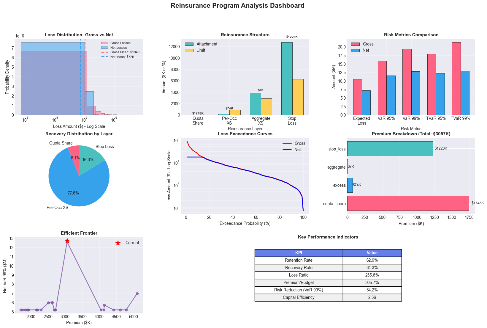
print("\n✨ OPTIMAL REINSURANCE STRUCTURE:")
print(f" • Quota Share: {optimal_structure.quota_share*100:.1f}%")
print(f" • XS: ${optimal_structure.xs_limit/1e3:.0f}K xs ${optimal_structure.xs_retention/1e3:.0f}K")
print(f" • Aggregate: ${optimal_structure.agg_limit/1e3:.0f}K xs ${optimal_structure.agg_retention/1e3:.0f}K")
print(f" • Stop Loss: ${optimal_structure.stop_loss_limit/1e3:.0f}K xs ${optimal_structure.stop_loss_retention/1e3:.0f}K")
print("\n📈 RISK METRICS:")
print(f" • Expected Loss (Gross): ${metrics.expected_loss_gross/1e6:.2f}M")
print(f" • Expected Loss (Net): ${metrics.expected_loss_net/1e6:.2f}M")
print(f" • VaR 99% (Gross): ${metrics.var_99_gross/1e6:.2f}M")
print(f" • VaR 99% (Net): ${metrics.var_99_net/1e6:.2f}M")
print(f" • TVaR 99% (Gross): ${metrics.tvar_99_gross/1e6:.2f}M")
print(f" • TVaR 99% (Net): ${metrics.tvar_99_net/1e6:.2f}M")
print("\n💰 PREMIUM BREAKDOWN:")
for layer, premium in metrics.premium_breakdown.items():
if layer != 'total':
print(f" • {layer.replace('_', ' ').title()}: ${premium/1e3:.0f}K")
print(f" • TOTAL PREMIUM: ${metrics.premium_total/1e3:.0f}K")
print("\n🎯 PERFORMANCE INDICATORS:")
print(f" • Retention Rate: {metrics.retention_rate*100:.1f}%")
print(f" • Recovery Rate: {metrics.recovery_rate*100:.1f}%")
print(f" • Loss Ratio: {metrics.loss_ratio*100:.1f}%")
print(f" • Risk Reduction (VaR 99%): {metrics.risk_reduction_var99:.1f}%")
print("\n✅ Analysis complete!")
Sample Output
================================================================================
ENHANCED REINSURANCE PROGRAM OPTIMIZER
Property & Casualty Insurance
================================================================================

📊 SIMULATION PARAMETERS:
  • Number of loss events: 1,000
  • Premium budget: $1,000,000
  • Loss distribution: Lognormal
  • Mean loss per event: $100,000
  • Coefficient of variation: 2.0

🎲 Generating loss scenarios...
  ✓ Generated 1,000 loss events
  ✓ Total losses: $103.9M
  ✓ Average loss: $104K
  ✓ Maximum loss: $5.93M

🔧 Optimizing reinsurance structure...

✨ OPTIMAL REINSURANCE STRUCTURE:
  • Quota Share: 2.2%
  • XS: $851K xs $169K
  • Aggregate: $2873K xs $3871K
  • Stop Loss: $6281K xs $12766K

📈 RISK METRICS:
  • Expected Loss (Gross): $10.54M
  • Expected Loss (Net): $7.21M
  • VaR 99% (Gross): $19.40M
  • VaR 99% (Net): $12.77M
  • TVaR 99% (Gross): $21.38M
  • TVaR 99% (Net): $12.98M

💰 PREMIUM BREAKDOWN:
  • Quota Share: $1748K
  • Excess: $74K
  • Aggregate: $7K
  • Stop Loss: $1228K
  • TOTAL PREMIUM: $3057K

🎯 PERFORMANCE INDICATORS:
  • Retention Rate: 62.9%
  • Recovery Rate: 34.3%
  • Loss Ratio: 235.8%
  • Risk Reduction (VaR 99%): 34.2%

✅ Analysis complete!
Practical Applications
Application: Portfolio Insurance

import numpy as np
import pandas as pd
from scipy import stats
from scipy.optimize import minimize_scalar

def portfolio_insurance_optimization(portfolio_value=100_000_000, n_years=10, n_sims=10000):
    """
    Demonstrate insurance mathematics concepts for portfolio protection:
    1. Frequency-severity modeling of market events
    2. Layer structuring (retention, primary, excess)
    3. Ergodic optimization (time-average growth vs ensemble average)
    4. Dynamic retention optimization based on wealth level
    """

    # 1. FREQUENCY-SEVERITY MODEL FOR MARKET EVENTS
    # Frequency: Number of adverse events per year (Poisson)
    event_frequency = stats.poisson(mu=2.5)  # Average 2.5 events/year

    # Severity: Size of loss given event (mixture for tail risk)
    # Small corrections: Log-normal
    small_severity = stats.lognorm(s=0.5, scale=0.03)  # 3% mean, moderate vol
    # Large crises: Pareto for heavy tails
    large_severity = stats.pareto(b=2.5, scale=0.10)  # Power law tail

    # Probability of large event given any event
    prob_large = 0.15

    # 2. INSURANCE LAYER STRUCTURE
    def calculate_layer_premiums(retention, primary_limit, excess_limit):
        """Calculate premiums for each layer using exposure curves."""
        base_rate = 0.015  # Base premium rate

        # Retention layer: Self-insured, no premium
        retention_premium = 0

        # Primary layer: Higher frequency, lower severity
        primary_rate = base_rate * (1 - np.exp(-primary_limit/retention))
        primary_premium = portfolio_value * primary_rate

        # Excess layer: Lower frequency, higher severity
        excess_rate = base_rate * 0.3 * (1 - np.exp(-excess_limit/primary_limit))
        excess_premium = portfolio_value * excess_rate

        return retention_premium, primary_premium, excess_premium

    # 3. SIMULATE PORTFOLIO PATHS WITH AND WITHOUT INSURANCE
    def simulate_wealth_path(initial_wealth, retention_pct, primary_pct, excess_pct,
                            use_insurance=True):
        """Simulate wealth evolution over multiple years."""
        wealth = initial_wealth
        wealth_history = [wealth]

        for year in range(n_years):
            # Base return (drift)
            base_return = 0.08
            normal_volatility = 0.15

            # Generate base portfolio return
            annual_return = np.random.normal(base_return, normal_volatility)

            # Generate adverse events (frequency-severity)
            n_events = event_frequency.rvs()
            total_event_loss = 0

            for _ in range(n_events):
                if np.random.rand() < prob_large:
                    # Large event (Pareto distributed)
                    loss = min(large_severity.rvs(), 0.5)  # Cap at 50% loss
                else:
                    # Small event (Log-normal distributed)
                    loss = min(small_severity.rvs(), 0.2)  # Cap at 20% loss
                total_event_loss += loss

            # Apply losses to portfolio
            gross_return = annual_return - total_event_loss

            if use_insurance:
                # Calculate insurance structure based on current wealth
                retention = wealth * retention_pct
                primary_limit = wealth * primary_pct
                excess_limit = wealth * excess_pct

                # Calculate premiums
                _, primary_prem, excess_prem = calculate_layer_premiums(
                    retention, primary_limit, excess_limit
                )
                total_premium = (primary_prem + excess_prem)

                # Apply insurance layers
                portfolio_loss = wealth * max(gross_return, -1.0)
                if portfolio_loss < 0:
                    loss_amount = abs(portfolio_loss)

                    # Retention (deductible)
                    retained_loss = min(loss_amount, retention)
                    remaining_loss = max(0, loss_amount - retention)

                    # Primary layer coverage
                    primary_recovery = min(remaining_loss, primary_limit)
                    remaining_loss = max(0, remaining_loss - primary_limit)

                    # Excess layer coverage
                    excess_recovery = min(remaining_loss, excess_limit)

                    # Net loss after insurance
                    net_loss = retained_loss + max(0, remaining_loss - excess_limit)
                    net_return = -net_loss / wealth
                else:
                    net_return = gross_return

                # Apply return and subtract premium
                wealth = wealth * (1 + net_return) - total_premium
            else:
                # No insurance - full exposure
                wealth = wealth * (1 + gross_return)

            # Ensure non-negative wealth
            wealth = max(0, wealth)
            wealth_history.append(wealth)

            # Stop if ruined
            if wealth == 0:
                break

        return wealth_history

    # 4. OPTIMIZE RETENTION USING ERGODIC PRINCIPLE
    def optimize_retention(initial_wealth):
        """Find optimal retention that maximizes time-average growth rate."""

        def negative_growth_rate(retention_pct):
            """Calculate negative of expected log growth rate."""
            if retention_pct < 0.01 or retention_pct > 0.5:
                return 1e6

            # Fixed layer structure for optimization
            primary_pct = min(0.15, (1 - retention_pct) * 0.5)
            excess_pct = min(0.25, (1 - retention_pct) * 0.8)

            # Simulate multiple paths
            final_wealths = []
            for _ in range(1000):  # Fewer sims for optimization
                path = simulate_wealth_path(
                    initial_wealth, retention_pct, primary_pct, excess_pct, True
                )
                if path[-1] > 0:
                    final_wealths.append(path[-1])

            if len(final_wealths) == 0:
                return 1e6

            # Calculate time-average growth rate
            growth_rates = [np.log(w / initial_wealth) / n_years
                            for w in final_wealths if w > 0]

            # Return negative for minimization
            return -np.mean(growth_rates) if growth_rates else 1e6

        # Optimize retention percentage
        result = minimize_scalar(
            negative_growth_rate,
            bounds=(0.01, 0.30),
            method='bounded',
            options={'xatol': 0.01}
        )

        return result.x

    # 5. RUN COMPREHENSIVE ANALYSIS
    print("=" * 60)
    print("PORTFOLIO INSURANCE OPTIMIZATION ANALYSIS")
    print("=" * 60)

    # Find optimal retention
    print("\n1. OPTIMAL RETENTION ANALYSIS")
    optimal_retention = optimize_retention(portfolio_value)
    print(f"   Optimal retention: {optimal_retention:.1%} of portfolio value")
    print(f"   Dollar amount: ${portfolio_value * optimal_retention:,.0f}")

    # Set insurance structure based on optimization
    retention_pct = optimal_retention
    primary_pct = min(0.15, (1 - retention_pct) * 0.5)
    excess_pct = min(0.25, (1 - retention_pct) * 0.8)

    print(f"\n2. OPTIMIZED LAYER STRUCTURE")
    print(f"   Retention:     0 - {retention_pct:.1%} (${portfolio_value*retention_pct:,.0f})")
    print(f"   Primary:       {retention_pct:.1%} - {retention_pct+primary_pct:.1%} (${portfolio_value*primary_pct:,.0f})")
    print(f"   Excess:        {retention_pct+primary_pct:.1%} - {retention_pct+primary_pct+excess_pct:.1%} (${portfolio_value*excess_pct:,.0f})")

    # Calculate premiums
    _, primary_prem, excess_prem = calculate_layer_premiums(
        portfolio_value * retention_pct,
        portfolio_value * primary_pct,
        portfolio_value * excess_pct
    )

    print(f"\n3. ANNUAL PREMIUM BREAKDOWN")
    print(f"   Primary layer:  ${primary_prem:,.0f} ({primary_prem/portfolio_value:.2%})")
    print(f"   Excess layer:   ${excess_prem:,.0f} ({excess_prem/portfolio_value:.2%})")
    print(f"   Total premium:  ${primary_prem + excess_prem:,.0f} ({(primary_prem + excess_prem)/portfolio_value:.2%})")

    # Run full simulation
    print(f"\n4. MONTE CARLO SIMULATION ({n_sims:,} paths, {n_years} years)")

    insured_paths = []
    uninsured_paths = []

    for _ in range(n_sims):
        # Insured portfolio
        insured = simulate_wealth_path(
            portfolio_value, retention_pct, primary_pct, excess_pct, True
        )
        insured_paths.append(insured[-1])

        # Uninsured portfolio
        uninsured = simulate_wealth_path(
            portfolio_value, 1.0, 0, 0, False
        )
        uninsured_paths.append(uninsured[-1])

    # Calculate statistics
    def calculate_metrics(values, initial):
        """Calculate key risk and return metrics."""
        values = np.array(values)
        positive_values = values[values > 0]

        if len(positive_values) == 0:
            return {
                'Mean': 0,
                'Median': 0,
                'Std Dev': 0,
                '5% VaR': initial,
                '1% CVaR': initial,
                'Ruin Prob': 1.0,
                'Growth Rate': -np.inf
            }

        # Time-average growth rate (ergodic)
        growth_rates = [np.log(v / initial) / n_years for v in positive_values]

        return {
            'Mean': np.mean(values),
            'Median': np.median(values),
            'Std Dev': np.std(values),
            '5% VaR': initial - np.percentile(values, 5),
            '1% CVaR': initial - np.mean(values[values <= np.percentile(values, 1)]),
            'Ruin Prob': np.mean(values <= 0),
            'Growth Rate': np.mean(growth_rates) if growth_rates else -np.inf
        }

    insured_metrics = calculate_metrics(insured_paths, portfolio_value)
    uninsured_metrics = calculate_metrics(uninsured_paths, portfolio_value)

    # Create comparison table
    comparison = pd.DataFrame({
        'Uninsured': list(insured_metrics.values()),
        'Insured': list(insured_metrics.values())
    }, index=insured_metrics.keys())

    print("\n5. RESULTS COMPARISON")
    print("-" * 60)

    results = []
    for metric in insured_metrics.keys():
        unins_val = uninsured_metrics[metric]
        ins_val = insured_metrics[metric]

        if metric in ['Mean', 'Median', 'Std Dev', '5% VaR', '1% CVaR']:
            results.append({
                'Metric': metric,
                'Uninsured': f"${unins_val:,.0f}",
                'Insured': f"${ins_val:,.0f}"
            })
        elif metric == 'Ruin Prob':
            results.append({
                'Metric': metric,
                'Uninsured': f"{unins_val:.2%}",
                'Insured': f"{ins_val:.2%}"
            })
        else:  # Growth Rate
            results.append({
                'Metric': 'Time-Avg Growth',
                'Uninsured': f"{unins_val:.2%}",
                'Insured': f"{ins_val:.2%}"
            })

    results_df = pd.DataFrame(results)
    print(results_df.to_string(index=False))

    # Key insights
    print("\n6. KEY INSIGHTS")
    print("-" * 60)
    print(f"✓ Insurance reduces ruin probability by {(uninsured_metrics['Ruin Prob'] - insured_metrics['Ruin Prob']):.1%}")
    print(f"✓ Time-average growth improved by {(insured_metrics['Growth Rate'] - uninsured_metrics['Growth Rate'])*100:.1f}bps")
    print(f"✓ Tail risk (1% CVaR) reduced by ${(uninsured_metrics['1% CVaR'] - insured_metrics['1% CVaR'])/1e6:.1f}M")
    print(f"✓ Optimal retention balances premium cost vs risk retention")

    return results_df

# Run the analysis
results = portfolio_insurance_optimization(
    portfolio_value=100_000_000,
    n_years=10,
    n_sims=5000  # Reduce for faster execution
)
Sample Output
============================================================
PORTFOLIO INSURANCE OPTIMIZATION ANALYSIS
============================================================

1. OPTIMAL RETENTION ANALYSIS
   Optimal retention: 1.6% of portfolio value
   Dollar amount: $1,617,301

2. OPTIMIZED LAYER STRUCTURE
   Retention:     0 - 1.6% ($1,617,301)
   Primary:       1.6% - 16.6% ($15,000,000)
   Excess:        16.6% - 41.6% ($25,000,000)

3. ANNUAL PREMIUM BREAKDOWN
   Primary layer:  $1,499,859 (1.50%)
   Excess layer:   $365,006 (0.37%)
   Total premium:  $1,864,865 (1.86%)

4. MONTE CARLO SIMULATION (5,000 paths, 10 years)

5. RESULTS COMPARISON
------------------------------------------------------------
         Metric   Uninsured      Insured
           Mean $60,021,752 $122,654,929
         Median $49,754,072 $114,719,654
        Std Dev $43,522,383  $43,328,475
         5% VaR $87,719,760  $31,093,881
        1% CVaR $97,415,436  $61,322,870
      Ruin Prob       0.20%        0.00%
Time-Avg Growth      -7.61%        1.47%

6. KEY INSIGHTS
------------------------------------------------------------
✓ Insurance reduces ruin probability by 0.2%
✓ Time-average growth improved by 9.1bps
✓ Tail risk (1% CVaR) reduced by $36.1M
✓ Optimal retention balances premium cost vs risk retention
Key Takeaways
Claims develop over time: Reserve adequacy is crucial
Frequency-severity framework is the foundation of insurance modeling
Multiple premium principles: Different approaches for different risks
Heavy tails matter: Extreme events dominate risk
Retention optimization balances premium savings with risk tolerance
Layers reduce cost: Structured coverage optimizes premium spend
Reinsurance complexity: Multiple structures serve different purposes
Next Steps
Chapter 4: Optimization Theory - Mathematical optimization methods
Chapter 5: Statistical Methods - Validation and testing
Chapter 1: Ergodic Economics - Foundational concepts