Multiplicative Processes in Finance and Insurance
🎯 Why This Matters
Multiplicative processes reveal why volatility is costly even when expected returns are unchanged: the volatility drag effect means a 30% volatility with 10% average return underperforms a steady 10% return due to compounding asymmetry. For P&C actuaries, this framework transforms how we value insurance: beyond covering expected losses, insurance creates value by reducing volatility drag, enabling higher sustainable growth rates. The Kelly criterion provides the mathematical foundation for optimal retention decisions, showing that maximizing log-wealth growth naturally prevents ruin while optimizing long-term performance. Path dependence explains why claims history, experience rating, and capital requirements can't be reduced to simple point estimates; the entire trajectory matters. These mathematics prove that smooth, predictable cash flows are inherently more valuable than volatile ones with the same mean, justifying insurance premiums that exceed expected losses and explaining why diversification and reinsurance remain rational even when they reduce expected returns.
Table of Contents

Introduction to Multiplicative Dynamics
Definition
A multiplicative process is one where changes are proportional to the current state:
where \(R_t\) is a random growth factor. This contrasts with additive processes:
where \(A_t\) is a random increment.
Why Multiplicative Processes Matter
Most economic quantities evolve multiplicatively:
Wealth: Returns compound on existing capital
Populations: Growth rates apply to current size
Company revenues: Growth percentages, not fixed amounts
Insurance losses: Often proportional to exposure
Key Properties
Non-negative: Cannot go below zero (natural boundary)
Scale-dependent: Absolute changes depend on current level
Compound effects: Small differences accumulate exponentially
Log-additivity: Logarithms transform to additive process
Geometric Brownian Motion
Mathematical Definition
Geometric Brownian Motion (GBM) is the continuous-time limit of multiplicative random walks:
\(S_t\) = Stock price or wealth at time \(t\)
\(\mu\) = Drift parameter (expected return)
\(\sigma\) = Volatility parameter
\(W_t\) = Standard Brownian motion
Analytical Solution
The solution to the GBM stochastic differential equation is:
This shows explicitly the volatility drag term \(-\sigma^2/2\).
Properties of GBM
Log-normality: \(\ln(S_t/S_0)\) is normally distributed
Martingale property: Under risk-neutral measure with \(\mu = r\) (risk-free rate)
Self-similarity: Statistical properties scale with time
Markov property: Future depends only on present, not past
Simulation in Discrete Time
Euler-Maruyama discretization for time step \(\Delta t\):
import matplotlib.pyplot as plt
import numpy as np

def simulate_gbm(S0, mu, sigma, T, dt, n_paths=1000):
    """Simulate Geometric Brownian Motion paths."""
    n_steps = int(T / dt)
    t = np.linspace(0, T, n_steps + 1)

        # Generate random shocks
    dW = np.random.randn(n_paths, n_steps) * np.sqrt(dt)

        # Initialize paths

    S = np.zeros((n_paths, n_steps + 1))
    S[:, 0] = S0

        # Simulate using exact solution for each step
    for i in range(n_steps):
        S[:, i + 1] = S[:, i] * np.exp((mu - 0.5 * sigma**2) * dt + sigma * dW[:, i])

    return t, S

# Example simulation
t, paths = simulate_gbm(S0=100, mu=0.08, sigma=0.2, T=10, dt=0.01)

plt.figure(figsize=(10, 6))
n_plot = min(10, paths.shape[0])  # plot up to 100 paths for readability
plt.plot(t, paths[:n_plot].T, lw=0.8, alpha=0.6)
plt.plot(t, paths.mean(axis=0), color='blue', lw=2, label='Mean path')
plt.xlabel('Time')
plt.ylabel('Price')
plt.title('Simulated GBM paths')
plt.legend()
plt.grid(True)
plt.show()

# Calculate statistics
final_values = paths[:, -1]
print(f"Mean final value: {np.mean(final_values):.2f}")
print(f"Median final value: {np.median(final_values):.2f}")
print(f"Probability of loss: {np.mean(final_values < 100):.1%}")
Sample Output
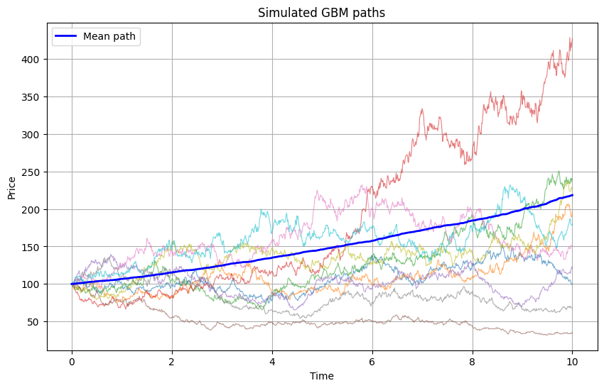
Mean final value: 218.46
Median final value: 178.65
Probability of loss: 18.3%
Log-Normal Distributions
Definition and Properties
If \(X \sim \text{LogNormal}(\mu, \sigma^2)\), then \(\ln(X) \sim \text{Normal}(\mu, \sigma^2)\).
Probability density function:
Moments of Log-Normal Distribution
For \(X \sim \text{LogNormal}(\mu, \sigma^2)\):
Mean: \(E[X] = e^{\mu + \sigma^2/2}\)
Median: \(\text{Med}[X] = e^{\mu}\)
Mode: \(\text{Mode}[X] = e^{\mu - \sigma^2}\)
Variance: \(\text{Var}[X] = e^{2\mu + \sigma^2}(e^{\sigma^2} - 1)\)
Note: Mean > Median > Mode (right-skewed distribution)
Connection to Multiplicative Processes
If returns are multiplicative with log-normal distribution:
Then wealth after \(n\) periods:
Taking logarithms:
By Central Limit Theorem, \(\ln(W_n)\) approaches normal distribution.
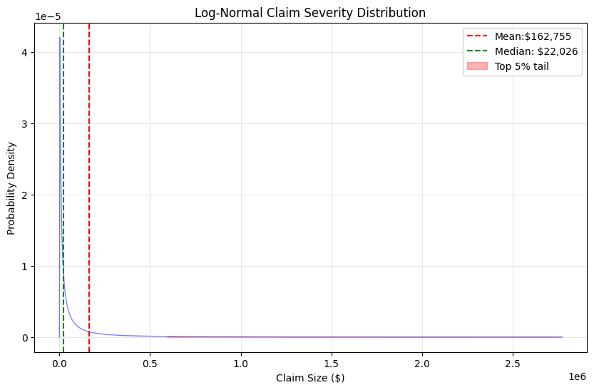
Insurance Loss Modeling
Log-normal distributions are common for:
Claim severities: Natural for multiplicative effects
Asset values: Result of compound growth
Time-to-event: With log-time normally distributed
from scipy import stats
import matplotlib.pyplot as plt

# Parameters for claim severity
mu_claim = 10  # log-mean (corresponds to ~$22k median)
sigma_claim = 2  # log-standard deviation

# Create distribution
claim_dist = stats.lognorm(s=sigma_claim, scale=np.exp(mu_claim))

# Calculate statistics
mean_claim = claim_dist.mean()
median_claim = claim_dist.median()
percentile_95 = claim_dist.ppf(0.95)
percentile_99 = claim_dist.ppf(0.99)

print(f"Mean claim:${mean_claim:,.0f}")
print(f"Median claim: ${median_claim:,.0f}")
print(f"95th percentile:${percentile_95:,.0f}")
print(f"99th percentile: ${percentile_99:,.0f}")

# Visualize
x = np.linspace(0, percentile_99 * 1.2, 1000)
pdf = claim_dist.pdf(x)

plt.figure(figsize=(10, 6))
plt.plot(x, pdf, 'b-', linewidth=2)
plt.axvline(mean_claim, color='r', linestyle='--', label=f'Mean:${mean_claim:,.0f}')
plt.axvline(median_claim,
    color='g',
    linestyle='--',
    label=f'Median: ${median_claim:,.0f}')
plt.fill_between(x[x > percentile_95],
    pdf[x > percentile_95],
    alpha=0.3,
    color='red',
    label='Top 5% tail')
plt.xlabel('Claim Size ($)')
plt.ylabel('Probability Density')
plt.title('Log-Normal Claim Severity Distribution')
plt.legend()
plt.grid(True, alpha=0.3)
plt.show()
Sample Output
Mean claim:$162,755
Median claim: $22,026
95th percentile:$591,080
99th percentile: $2,309,856
Path Dependence and History
Definition of Path Dependence
A process is path-dependent if the outcome depends not just on the starting and ending points, but on the entire trajectory taken.
Examples in Finance
Bankruptcy: Once wealth hits zero, it stays there
Credit ratings: History of defaults affects future borrowing
Barrier options: Payoff depends on whether price crossed a threshold
Asian options: Payoff based on average price over time
Mathematical Formulation
For a path-dependent functional:
Cannot be reduced to:
Impact on Insurance
Path dependence affects:
Claims development: Past payments influence reserves
Experience rating: History determines future premiums
Reputation effects: Past performance affects market position
Capital requirements: Regulatory views based on history
Measuring Path Dependence
# First run the GMB example above to generate `paths`

def calculate_path_metrics(paths):
    """Calculate various path-dependent metrics."""

    metrics = {
        'final_value': paths[:, -1],
        'maximum': np.max(paths, axis=1),
        'minimum': np.min(paths, axis=1),
        'average': np.mean(paths, axis=1),
        'max_drawdown': np.zeros(len(paths)),
        'time_underwater': np.zeros(len(paths)),
        'volatility_realized': np.zeros(len(paths))
    }

    for i, path in enumerate(paths):
        # Maximum drawdown
        cummax = np.maximum.accumulate(path)
        drawdown = (cummax - path) / cummax
        metrics['max_drawdown'][i] = np.max(drawdown)

        # Time underwater
        metrics['time_underwater'][i] = np.mean(path < path[0])

        # Realized volatility
        returns = np.diff(np.log(path))
        metrics['volatility_realized'][i] = np.std(returns) * np.sqrt(252)

    return metrics

# Analyze path dependence
metrics = calculate_path_metrics(paths)

# Compare final values with path metrics
correlation_matrix = np.corrcoef([
    metrics['final_value'],
    metrics['maximum'],
    metrics['max_drawdown'],
    metrics['volatility_realized']
])

print("Correlation with final value:")
print(f"Maximum reached: {correlation_matrix[0, 1]:.3f}")
print(f"Max drawdown: {correlation_matrix[0, 2]:.3f}")
print(f"Realized volatility: {correlation_matrix[0, 3]:.3f}")
Sample Output
Correlation with final value:
Maximum reached: 0.962
Max drawdown: -0.604
Realized volatility: -0.001
Growth Rate Calculations
Suppose we have a multiplicative process:
Where \(R_t\) is a random growth factor at each period with expectation \(R\).
Two Different Questions We Can Ask:
1. Ensemble Average (Arithmetic Mean):
“What is the expected wealth across many people/paths at time \(T\)?”
Person 1: \(W_T^{(1)} = W_0 \cdot R_1^{(1)} \cdot R_2^{(1)} \cdot ... \cdot R_T^{(1)}\)
Person 2: \(W_T^{(2)} = W_0 \cdot R_1^{(2)} \cdot R_2^{(2)} \cdot ... \cdot R_T^{(2)}\)
…
Person N: \(W_T^{(N)} = W_0 \cdot R_1^{(N)} \cdot R_2^{(N)} \cdot ... \cdot R_T^{(N)}\)
The ensemble average is the expected value: \(E[W_T]_\text{ensemble} = \frac{1}{N}\sum_{i=1}^N{W_T^{(i)}}\)
As \(N \rightarrow \infin\), this converges to \(E[W_T] = W_0 \cdot E[R]^T\) (for i.i.d. returns).
And we have \(E[R] = 1 + r_a\)
2. Time Average (Geometric Mean):
“What growth rate does a single individual experience over time?”
For one specific path: \(W_T = W_0 \cdot R_1 \cdot R_2 \cdot ... \cdot R_T\)
The growth rate thus experienced is: \(g = (\frac{W_T}{W_0})^\frac{1}{T} - 1 = (\prod{R_t})^\frac{1}{T} - 1\)
As \(T \rightarrow \infin\), this converges to \(\langle g \rangle_\text{time} = \lim_{T \rightarrow \infin}{\frac{1}{T}\ln{\frac{W_T^{(i)}}{W_0}}} = E[\ln(R)]\)
And we have \(W_T = W_0 \cdot (1 + r_g)^T\)
Relationship Between Returns
For small returns, approximately:
Exact relationship:
Volatility Drag
The difference between arithmetic and geometric means:
This represents the cost of volatility on compound growth.
Example Calculation
def analyze_growth_rates(returns):
    """Compare different growth rate measures."""

    # Arithmetic mean
    r_arithmetic = np.mean(returns)

    # Geometric mean
    wealth_factor = np.prod(1 + returns)
    r_geometric = wealth_factor**(1/len(returns)) - 1

    # Log growth rate
    log_returns = np.log(1 + returns)
    g_log = np.mean(log_returns)

    # Volatility
    volatility = np.std(returns)

    # Theoretical drag
    theoretical_drag = volatility**2 / 2
    actual_drag = r_arithmetic - r_geometric

    results = {
    'Arithmetic Mean': r_arithmetic,
    'Geometric Mean': r_geometric,
    'Log Growth Rate': g_log,
    'Volatility': volatility,
    'Theoretical Drag': theoretical_drag,
    'Actual Drag': actual_drag,
    'Final Wealth Multiple': wealth_factor
    }

    return results

# Example with volatile returns
np.random.seed(42)
returns = np.random.randn(100) * 0.3 + 0.1
# 10% mean, 30% volatility

results = analyze_growth_rates(returns)
for key, value in results.items():
    if 'Wealth' in key:
        print(f"{key}: {value:.2f}x")
    else:
        print(f"{key}: {value:.2%}")
Sample Output
Arithmetic Mean: 6.88%
Geometric Mean: 2.97%
Log Growth Rate: 2.92%
Volatility: 27.11%
Theoretical Drag: 3.67%
Actual Drag: 3.92%
Final Wealth Multiple: 18.62x
The Kelly Criterion
What Is It?
The Kelly Criterion is a mathematical framework that answers a critical question: “How much risk is too much?”
Originally developed for gambling and investing, it determines the optimal size of bets (or in insurance terms, retentions) to maximize long-term growth while avoiding ruin.
The formula balances two competing forces:
Too much risk retention → Higher probability of catastrophic loss
Too much risk transfer → Excessive premiums erode profitability
Kelly identifies the sweet spot that maximizes compound growth rate over time, not just expected value in any single period. In essence, Kelly solves a specific problem in situations where Ergodicity breaks down (when time ≠ ensemble averages).
Original Formulation
For a binary bet with probability \(p\) of winning \(b\) times the wager:
where \(f^*\) is the optimal fraction of wealth to bet.
Continuous Distribution
For continuous returns \(R\) with distribution \(F\):
Where the \(\arg\max\limits_f\) function returns \(f\) that maximizes the expectation.
Insurance Application
Optimal retention level:
Properties of Kelly Betting
Maximizes geometric growth: Optimal for long-term wealth
Never risks ruin: Always maintains positive wealth
Volatility-adjusted: Naturally accounts for risk
Time-consistent: Optimal regardless of horizon
Fractional Kelly
Due to estimation error and preferences, practitioners often use fractional Kelly:
where \(\alpha \in (0, 1]\), typically \(\alpha \approx\) 0.25 to 0.5.
Implementation
from scipy.optimize import minimize_scalar


def kelly_optimal_insurance(wealth, growth_rate, volatility,
    claim_frequency, claim_severity_dist,
    premium_loading=1.3):
    """Find Kelly-optimal insurance retention."""

    def expected_log_wealth(retention):
        # Annual premium
        expected_loss = claim_frequency * claim_severity_dist.mean()
        premium = min(expected_loss, retention) * premium_loading

        # Simulate one year
        n_sims = 10_000
        final_wealth = np.zeros(n_sims)

        for i in range(n_sims):
            # Base growth
            w = wealth * np.exp(growth_rate - 0.5*volatility**2 + volatility*np.random.randn())

            # Claims
            n_claims = np.random.poisson(claim_frequency)

            if n_claims > 0:
                claims = claim_severity_dist.rvs(n_claims)
                total_claim = np.sum(claims)
                retained_loss = min(total_claim, retention)
            else:
                retained_loss = 0

            # Final wealth
            final_wealth[i] = max(0, w - premium - retained_loss)

            # Expected log wealth (excluding zeros)
            positive_wealth = final_wealth[final_wealth > 0]
            if len(positive_wealth) == 0:
                return -np.inf

        return np.mean(np.log(positive_wealth / wealth))

    # Optimize
    result = minimize_scalar(
        lambda r: -expected_log_wealth(r),
        bounds=(0, wealth * 0.5),
        method='bounded'
    )

    return result.x

# Example usage
claim_dist = stats.lognorm(s=2, scale=50000)
optimal_retention = kelly_optimal_insurance(
    wealth=10_000_000,
    growth_rate=0.08,
    volatility=0.15,
    claim_frequency=3,
    claim_severity_dist=claim_dist
)

print(f"Kelly-optimal retention: ${optimal_retention:,.0f}")
Sample Output
Kelly-optimal retention: $18,155
Volatility Drag
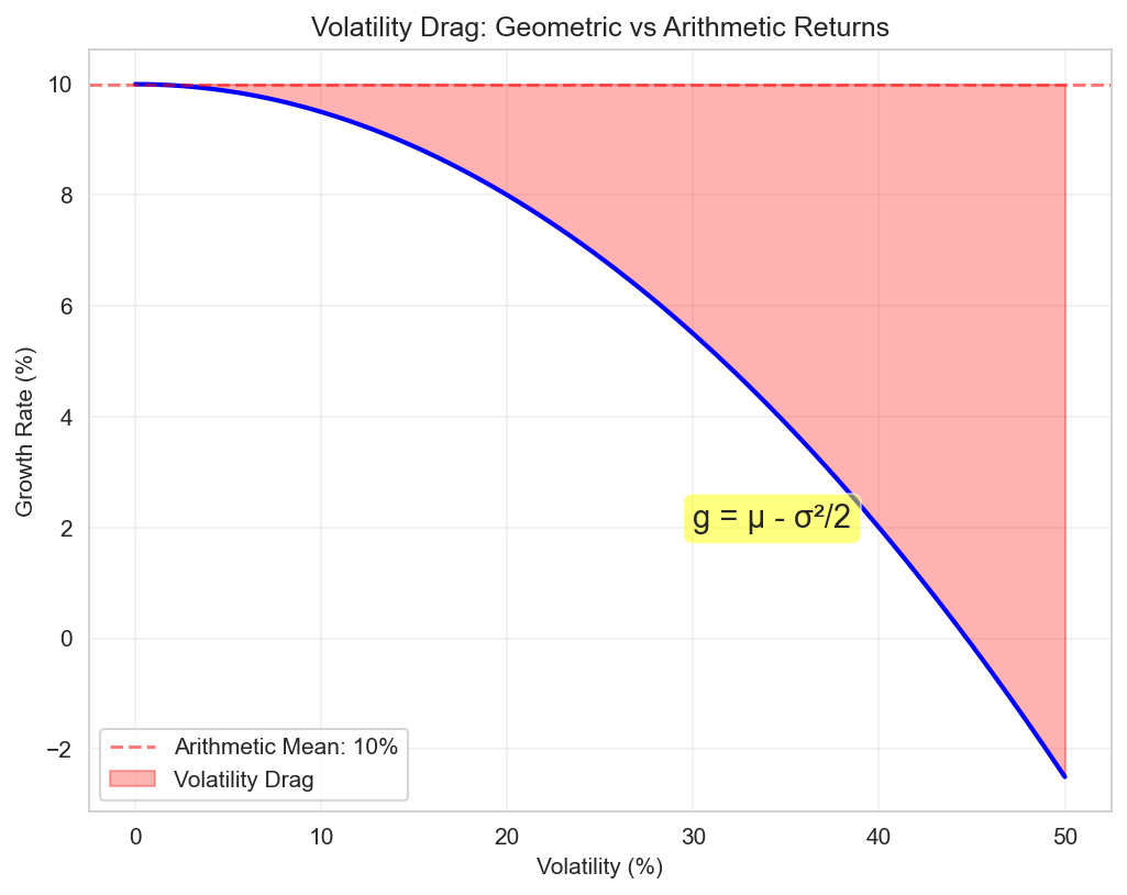
Figure: The impact of volatility on growth rates, showing how geometric mean decreases with volatility even when arithmetic mean is constant.
Mathematical Definition
For a process with arithmetic mean return \(\mu\) and volatility \(\sigma\):
This reduces the geometric growth rate:
Intuitive Explanation
Consider two scenarios:
Steady 10% annual return → \(1.1^{10} = 2.594x\) after 10 years
Alternating +30% and -10% (average 10%) → \((1.3 × 0.9)^5 = 2.373x\)
The volatile path underperforms despite the same average.
Impact on Insurance Decisions
Insurance reduces volatility drag by:
Capping downside losses
Smoothing cash flows
Enabling higher risk-taking in core business
Quantifying the Benefit
def calculate_volatility_drag_benefit(base_volatility,
                                     volatility_with_insurance,
                                     time_horizon=10):
    """Calculate wealth improvement from volatility reduction."""

    # Assume same arithmetic mean
    mu = 0.10

    # Growth rates
    g_without = mu - base_volatility**2 / 2
    g_with = mu - volatility_with_insurance**2 / 2

    # Wealth multiples
    wealth_without = np.exp(g_without * time_horizon)
    wealth_with = np.exp(g_with * time_horizon)

    # Benefit
    benefit = (wealth_with / wealth_without - 1) * 100

    print(f"Base volatility: {base_volatility:.1%}")
    print(f"Volatility with insurance: {volatility_with_insurance:.1%}")
    print(f"Growth without insurance: {g_without:.2%}")
    print(f"Growth with insurance: {g_with:.2%}")
    print(f"Wealth improvement: {benefit:.1f}%")

    return benefit

# Example
benefit = calculate_volatility_drag_benefit(
    base_volatility=0.30,
    volatility_with_insurance=0.15,
    time_horizon=20
)
Sample Output
Base volatility: 30.0%
Volatility with insurance: 15.0%
Growth without insurance: 5.50%
Growth with insurance: 8.88%
Wealth improvement: 96.4%
Practical Examples
Example 1: Widget Manufacturer

A widget manufacturer faces:
$10M starting capital
Revenue growth: 8% expected, 15% volatility
Operating leverage: 2x (costs are 50% fixed)
Catastrophic risk: 5% chance to lose 50% of capital
def simulate_manufacturer(years=10, with_insurance=False):
    """Simulate manufacturer wealth evolution."""

    W0 = 10_000_000  # \$10M initial capital
    wealth = [W0]

    for year in range(years):
        # Revenue growth
        revenue_shock = np.exp(0.08 - 0.5*0.15**2 + 0.15*np.random.randn())

        # Operating leverage effect
        profit_shock = 1 + 2 * (revenue_shock - 1)

        # Catastrophic loss
        cat_loss = wealth[-1] / 2.0
        cat_prob = 0.05
        if np.random.rand() < cat_prob:
            loss = cat_loss
        else:
            loss = 0

        if with_insurance:
            retention = 500_000
            premium = (cat_loss - retention) * cat_prob / 0.7  # 70% Loss Ratio
            covered_loss = max(0, loss - retention)
            net_loss = premium + min(loss, retention)
        else:
            net_loss = loss

        # Update wealth
        new_wealth = max(0, wealth[-1] * profit_shock - net_loss)
        wealth.append(new_wealth)

    return wealth

# Run simulations
np.random.seed(42)
n_sims = 100_000
results_with = []
results_without = []

for _ in range(n_sims):
    results_with.append(simulate_manufacturer(20, True))
    results_without.append(simulate_manufacturer(20, False))

# Analyze
final_with = [r[-1] for r in results_with]
final_without = [r[-1] for r in results_without]

fw = np.array(final_with)
fwo = np.array(final_without)

plt.figure(figsize=(10, 6))
plt.hist(fw, bins=100, density=True, alpha=0.5, label='With insurance')
plt.hist(fwo, bins=100, density=True, alpha=0.5, label='Without insurance')
plt.xscale('symlog', linthresh=1e3)  # show tails but keep visibility near zero
plt.xlabel('Final wealth ($)')
plt.ylabel('Density')
plt.title('Final wealth distributions: with vs without insurance')
plt.legend()
plt.grid(True, which='both', alpha=0.3)
plt.show()

print("With Insurance:")
print(f"  Median final wealth: ${np.median(final_with):,.0f}")
print(f"  Bankruptcy rate: {np.mean(np.array(final_with) == 0):.1%}")
print(f"  Growth rate: {np.mean(np.log(np.array(final_with)[np.array(final_with) > 0] / 10_000_000) / 20):.2%}")

print("\nWithout Insurance:")
print(f"  Median final wealth: ${np.median(final_without):,.0f}")
print(f"  Bankruptcy rate: {np.mean(np.array(final_without) == 0):.1%}")
print(f"  Growth rate: {np.mean(np.log(np.array(final_without)[np.array(final_without) > 0] / 10_000_000) / 20):.2%}")
Sample Output
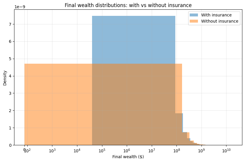
With Insurance:
  Median final wealth: $50,420,575
  Bankruptcy rate: 0.0%
  Growth rate: 7.98%

Without Insurance:
  Median final wealth: $54,126,214
  Bankruptcy rate: 0.9%
  Growth rate: 8.09%
Example 2: Investment Portfolio

Portfolio with tail risk:
Starting portfolio of $100M
Fixed operating costs of $500K per year
Base Return: 7% with 15% Volatility
Tail event: 2% chance of 40% loss
1.5x Leverage
Hedge option: protects downside below 20% at a price of 1.5% of assets
def portfolio_with_tail_risk(leverage=1.0, tail_hedge=False):
    """Simulate leveraged portfolio with tail risk."""

    # Parameters
    years = 30
    base_return = 0.07
    base_vol = 0.15
    tail_prob = 0.02  # 2% annual chance
    tail_loss = 0.40  # 40% loss in tail event

    fixed_costs = 500_000

    wealth_paths = []

    for _ in range(1000):
        wealth = 100_000_000
        for year in range(years):
            # Normal return with leverage
            normal_return = base_return * leverage
            normal_vol = base_vol * leverage

            year_return = np.random.randn() * normal_vol + normal_return

            # Tail event
            if np.random.rand() < tail_prob:
                year_return = -tail_loss * leverage

            if tail_hedge:
                # Pay 1.5% for tail protection
                hedge_cost = 0.015
                if year_return < -0.20:
                    year_return = -0.20  # Cap losses at 20%
                year_return -= hedge_cost

            wealth *= (1 + year_return)
            wealth -= fixed_costs
            wealth = max(0, wealth)

        wealth_paths.append(wealth)

    return np.array(wealth_paths)

# Compare strategies
unhedged = portfolio_with_tail_risk(leverage=1.5, tail_hedge=False)
hedged = portfolio_with_tail_risk(leverage=1.5, tail_hedge=True)

print("Leveraged Portfolio (1.5x):")
print(f"Without hedge - Median: ${np.median(unhedged):,.0f}; Ruin: {np.mean(unhedged == 0):.1%}")
print(f"   With hedge - Median: ${np.median(hedged):,.0f}; Ruin: {np.mean(hedged == 0):.1%}")
Sample Output
Leveraged Portfolio (1.5x):
Without hedge - Median: $551,012,310; Ruin: 0.6%
   With hedge - Median: $754,000,522; Ruin: 0.0%
Key Takeaways
Multiplicative processes dominate economics: most financial quantities compound
GBM captures essential features, but real processes have jumps and fat tails
Log-normal distributions arise naturally from multiplicative effects
Path dependence matters: history constrains future possibilities
Geometric mean < Arithmetic mean: volatility drag is real and substantial
Volatility reduction enhances growth: insurance benefit beyond loss coverage
Kelly criterion optimizes growth, providing a natural framework for insurance decisions
Next Steps
Chapter 1: Ergodic Economics - Foundational concepts
Chapter 3: Insurance Mathematics - Specific insurance applications
Chapter 4: Optimization Theory - Mathematical optimization methods