2. Basic Simulation Tutorial
This tutorial provides a comprehensive guide to running simulations with the Ergodic Insurance Framework. You’ll learn how to configure manufacturers, generate realistic losses, and run various simulation scenarios.
2.1. Learning Objectives
After completing this tutorial, you will be able to:
Configure manufacturer models with realistic parameters
Generate different types of loss distributions
Run Monte Carlo simulations
Analyze simulation results statistically
Visualize outcomes effectively
2.2. Setting Up a Manufacturer
The Manufacturer class models a company’s financial dynamics. Let’s explore its key parameters:
2.2.1. Basic Configuration
import numpy as np

from ergodic_insurance.manufacturer import WidgetManufacturer
from ergodic_insurance.config_v2 import ManufacturerConfig, WorkingCapitalConfig

# Create a medium-sized manufacturer
mfg_config = ManufacturerConfig(
    initial_assets=10_000_000,    # Starting with $10M
    asset_turnover_ratio=1.0,     # Generate revenue equal to assets
    base_operating_margin=0.12,        # Profit margin before losses
    tax_rate=0.25,                # 25% corporate tax
    retention_ratio=0.7           # Retain 70% of earnings
)

mfg_working_capital_config = WorkingCapitalConfig(
    percent_of_sales=0.20  # 20% of revenue tied up in WC
)

manufacturer = WidgetManufacturer(mfg_config, mfg_working_capital_config)

# Calculate key metrics
annual_revenue = manufacturer.assets * manufacturer.asset_turnover_ratio
operating_income = annual_revenue * manufacturer.base_operating_margin
net_income = operating_income * (1 - manufacturer.tax_rate)

print(f"Company Financial Profile:")
print(f"  Assets: ${manufacturer.assets:,.0f}")
print(f"  Annual Revenue: ${annual_revenue:,.0f}")
print(f"  Operating Income: ${operating_income:,.0f}")
print(f"  Net Income: ${net_income:,.0f}")
print(f"  ROA: {net_income / manufacturer.assets:.1%}")
2.2.1.1. Expected Output
Company Financial Profile:
  Assets: $10,000,000
  Annual Revenue: $10,000,000
  Operating Income: $1,200,000
  Net Income: $900,000
  ROA: 9.0%
2.2.2. Sector-Specific Configurations
Different manufacturing sectors have different financial characteristics:
import numpy as np

from ergodic_insurance.manufacturer import WidgetManufacturer
from ergodic_insurance.config_v2 import ManufacturerConfig

# Capital-intensive manufacturing
heavy_industry = WidgetManufacturer(ManufacturerConfig(
    initial_assets=50_000_000,
    asset_turnover_ratio=0.5,  # Low turnover
    base_operating_margin=0.05,     # 5% margins
    tax_rate=0.25,
    retention_ratio=0.7
))

# High-efficiency light manufacturer (e.g., consumer goods, textiles)
light_manufacturer = WidgetManufacturer(ManufacturerConfig(
    initial_assets=5_000_000,
    asset_turnover_ratio=2.0,  # High turnover - efficient asset use
    base_operating_margin=0.08,     # Moderate margins
    tax_rate=0.25,
    retention_ratio=0.6        # Lower retention due to distribution needs
))

# High-tech manufacturer (e.g., semiconductors, medical devices)
high_tech = WidgetManufacturer(ManufacturerConfig(
    initial_assets=25_000_000,  # Capital intensive
    asset_turnover_ratio=0.8,   # Moderate turnover
    base_operating_margin=0.35,       # High margins from IP/technology
    tax_rate=0.21,              # Lower effective tax rate
    retention_ratio=0.85        # High retention for R&D investment
))

# Compare profitability
for company, name in [
    (heavy_industry, "Heavy Industry"),
    (light_manufacturer, "Light Manufacturer"),
    (high_tech, "High-Tech")
]:
    revenue = company.assets * company.asset_turnover_ratio
    profit = revenue * company.base_operating_margin * (1 - company.tax_rate)
    roe = profit / company.assets
    print(f"{name}:")
    print(f"  Assets: ${company.assets:,.0f}")
    print(f"  Revenue: ${revenue:,.0f}")
    print(f"  ROE: {roe:.1%}")
    print()
2.2.2.1. Expected Output
Warning: Operating margin 35.0% is unusually high
Heavy Industry:
  Assets: $50,000,000
  Revenue: $25,000,000
  ROE: 1.9%

Light Manufacturer:
  Assets: $5,000,000
  Revenue: $10,000,000
  ROE: 12.0%

High-Tech:
  Assets: $25,000,000
  Revenue: $20,000,000
  ROE: 22.1%
2.3. Generating Losses
The ClaimGenerator creates realistic loss scenarios. Let’s explore different loss patterns:
2.3.1. Basic Loss Generation
import numpy as np

from ergodic_insurance.claim_generator import ClaimGenerator

# Standard loss generator
standard_losses = ClaimGenerator(
    base_frequency=5,
    severity_mean=80_000,
    severity_std=65_000
)

# Generate 5 years of losses
sim_years = 5
standard_losses.rng.seed(42)  # For reproducibility
losses_by_year = standard_losses.generate_claims(years=sim_years)
for year in range(sim_years):
    annual_losses = [loss for loss in losses_by_year if loss.year == year]
    annual_total = sum(loss.amount for loss in annual_losses)
    print(f"Year {year+1}: {len(annual_losses)} losses, Total: ${annual_total:,.0f}")
2.3.1.1. Sample Output
Year 1: 5 losses, Total: $478,808
Year 2: 5 losses, Total: $328,959
Year 3: 3 losses, Total: $148,976
Year 4: 4 losses, Total: $210,324
Year 5: 9 losses, Total: $488,578
2.3.2. Different Risk Profiles
from ergodic_insurance.claim_generator import ClaimGenerator

# Low frequency, high severity (catastrophic risk)
catastrophic_risk = ClaimGenerator(
    base_frequency=0.1,         # One loss every 10 years
    severity_mean=1_000_000,      # Much larger losses
    severity_std=500_000     # More variability
)

# High frequency, low severity (operational risk)
operational_risk = ClaimGenerator(
    base_frequency=20,          # Many small losses
    severity_mean=3_000,       # Smaller losses
    severity_std=1_000     # Less variability
)

# Simulate and compare
np.random.seed(42)
years = 10
risk_profiles = {
    "Standard": standard_losses,
    "Catastrophic": catastrophic_risk,
    "Operational": operational_risk
}

all_losses = []
for name, generator in risk_profiles.items():
    generator_losses = []
    for year in range(years):
        generator.rng.seed(42 + year)  # Different seed each year
        annual = generator.generate_year(year=year)
        generator_losses.extend(annual)

    if generator_losses:
        print(f"\n{name} Risk Profile ({years} years):")
        print(f"  Total losses: {len(generator_losses)}")
        print(f"  Average loss: ${np.mean([loss.amount for loss in generator_losses]):,.0f}")
        print(f"  Largest loss: ${max(loss.amount for loss in generator_losses):,.0f}")
        print(f"  Total amount: ${sum(loss.amount for loss in generator_losses):,.0f}")

    all_losses.extend(generator_losses)
2.3.2.1. Sample Output
Standard Risk Profile (10 years):
  Total losses: 46
  Average loss: $76,491
  Largest loss: $233,220
  Total amount: $3,518,578

Catastrophic Risk Profile (10 years):
  Total losses: 4
  Average loss: $1,075,799
  Largest loss: $1,614,911
  Total amount: $4,303,197

Operational Risk Profile (10 years):
  Total losses: 202
  Average loss: $2,936
  Largest loss: $8,345
  Total amount: $593,058
2.4. Running Simulations
Now let’s run comprehensive simulations with different scenarios:
2.4.1. Single Path Simulation
from ergodic_insurance.insurance import InsurancePolicy, InsuranceLayer
from ergodic_insurance.simulation import Simulation

### Using previously defined manufacturer and losses #######

# Policy parameters
deductible = 200_000
limit = 40_000_000

### Calculate a fair premium #######
# Calculate pure premium
total_covered_losses = sum(min(max(0, loss.amount - deductible), limit) \
                            for loss in all_losses)
pure_premium = total_covered_losses / years  # As a fraction of assets
loss_ratio = 0.70  # 70% of premiums go towards losses
reasonable_premium = pure_premium / loss_ratio
reasonable_rate = reasonable_premium / limit
print(f"Calculated Reasonable Premium: ${reasonable_premium:,.0f}")

### Set up the policy #######
single_layer = InsuranceLayer(
    attachment_point=deductible,
    limit=limit,
    rate=reasonable_rate
)

insurance_policy = InsurancePolicy(
    layers=[single_layer],
    deductible=deductible
)

### Set up the simulation #######
sim = Simulation(
    manufacturer=heavy_industry,
    claim_generator=[standard_losses, catastrophic_risk, operational_risk],
    insurance_policy=insurance_policy,
    time_horizon=20,  # 20-year simulation
    seed=42
)

results = sim.run()
result_summary = results.summary_stats()

print(f"20-Year Simulation Results:")
print(f"Starting Assets: ${heavy_industry.config.initial_assets:,.0f}")
print(f"Final Assets: ${result_summary['final_assets']:,.0f}")
print(f"Final Assets: ${result_summary['final_assets']:,.0f}")
print(f"Time-Weighted ROE: {result_summary['time_weighted_roe']:.2%}")
2.4.1.1. Sample Output
Calculated Reasonable Premium: $85,661
20-Year Simulation Results:
Starting Assets: $50,000,000
Final Assets: $53,379,921
Final Assets: $53,379,921
Time-Weighted ROE: 1.82%
2.4.2. Monte Carlo Simulation
For robust analysis, we need multiple simulation paths:
from ergodic_insurance.monte_carlo import MonteCarloEngine, SimulationConfig
from ergodic_insurance.insurance_program import InsuranceProgram, EnhancedInsuranceLayer
from ergodic_insurance.loss_distributions import ManufacturingLossGenerator

# Create a ManufacturingLossGenerator for Monte Carlo simulation
# (MonteCarloEngine expects this type, not ClaimGenerator)
mc_loss_generator = ManufacturingLossGenerator(
    attritional_params={
        'base_frequency': 3.0,  # Similar to standard_losses frequency
        'severity_mean': 40_000,  # Similar to standard_losses severity
        'severity_cv': 0.8  # Coefficient of variation
    },
    large_params={
        'base_frequency': 0.1,  # Occasional large losses
        'severity_mean': 500_000,
        'severity_cv': 1.2
    },
    seed=42
)

# Create insurance program with enhanced layers
# EnhancedInsuranceLayer has the required methods for InsuranceProgram
insurance_layers = [
    EnhancedInsuranceLayer(
        attachment_point=100_000,    # $100K deductible
        limit=10_000_000,            # $10M limit
        base_premium_rate=0.015            # 2% rate on limit
    )
]
insurance_program = InsuranceProgram(layers=insurance_layers)

# Configure Monte Carlo simulation
mc_config = SimulationConfig(
    n_simulations=1000,
    n_years=20,
    parallel=False,  # Set to False for simpler execution
    progress_bar=True,
    seed=42
)

# Create Monte Carlo engine
mc_engine = MonteCarloEngine(
    loss_generator=mc_loss_generator,
    insurance_program=insurance_program,
    manufacturer=heavy_industry,
    config=mc_config
)

# Run simulations
print("Running Monte Carlo simulations...")
mc_results = mc_engine.run()

# Extract results
survival_rate = 1 - mc_results.ruin_probability
mean_growth = np.mean(mc_results.growth_rates)
median_growth = np.median(mc_results.growth_rates)
var_95 = np.percentile(mc_results.growth_rates, 5)
mean_final_assets = np.mean(mc_results.final_assets)

print(f"\nMonte Carlo Results (1000 simulations):")
print(f"  Survival Rate: {survival_rate:.1%}")
print(f"  Mean Growth Rate: {mean_growth:.2%}")
print(f"  Median Growth Rate: {median_growth:.2%}")
print(f"  95% VaR Growth: {var_95:.2%}")
print(f"  Starting Wealth: ${mc_engine.manufacturer._initial_assets:,.0f}")
print(f"  Mean Final Wealth: ${mean_final_assets:,.0f}")
2.4.2.1. Sample Output
Monte Carlo Results (1000 simulations):
  Survival Rate: 100.0%
  Mean Growth Rate: 0.51%
  Median Growth Rate: 0.56%
  95% VaR Growth: 0.03%
  Starting Wealth: $50,000,000
  Mean Final Wealth: $59,211,744
2.4.3. Comparing Insurance Strategies
# Define different insurance strategies
strategies = [
    {"name": "No Insurance", "attachment": float('inf'), "limit": 0, "base_premium_rate": 0},
    {"name": "High Deductible", "attachment": 2_000_000, "limit": 10_000_000, "base_premium_rate": 0.01},
    {"name": "Medium Coverage", "attachment": 500_000, "limit": 5_000_000, "base_premium_rate": 0.015},
    {"name": "Full Coverage", "attachment": 100_000, "limit": 20_000_000, "base_premium_rate": 0.02}
]

# Run simulations for each strategy
results_comparison = {}

for strategy in strategies:
    # Create insurance layers for this strategy
    if strategy['limit'] > 0:
        strategy_layers = [
            EnhancedInsuranceLayer(
                attachment_point=strategy['attachment'],
                limit=strategy['limit'],
                base_premium_rate=strategy['base_premium_rate']
            )
        ]
        strategy_insurance = InsuranceProgram(layers=strategy_layers)
    else:
        # No insurance case
        strategy_insurance = InsuranceProgram(layers=[])

    # Configure simulation for this strategy
    strategy_config = SimulationConfig(
        n_simulations=500,
        n_years=20,
        parallel=False,
        progress_bar=False,  # Disable for cleaner output
        seed=42
    )

    # Create new engine for this strategy
    strategy_engine = MonteCarloEngine(
        loss_generator=mc_loss_generator,
        insurance_program=strategy_insurance,
        manufacturer=heavy_industry.copy(),  # Use a copy to ensure independence
        config=strategy_config
    )

    # Run simulations
    print(f"Running {strategy['name']}...")
    strategy_results = strategy_engine.run()
    results_comparison[strategy['name']] = strategy_results

# Compare strategies
print("\nStrategy Comparison:")
print(f"{'Strategy':<20} {'Survival':<12} {'Mean Growth':<12} {'Volatility':<12}")
print("-" * 56)

for name, results in results_comparison.items():
    survival = 1 - results.ruin_probability
    mean_growth = np.mean(results.growth_rates)
    vol = np.std(results.growth_rates)
    print(f"{name:<20} {survival:>10.1%}   {mean_growth:>10.2%}   {vol:>10.2%}")
2.4.3.1. Sample Output
Strategy Comparison:
Strategy             Survival     Mean Growth  Volatility
--------------------------------------------------------
No Insurance             100.0%        0.98%        0.26%
High Deductible          100.0%        0.90%        0.32%
Medium Coverage          100.0%        0.94%        0.22%
Full Coverage            100.0%        0.59%        0.31%
2.5. Visualizing Results
Effective visualization helps understand simulation outcomes:
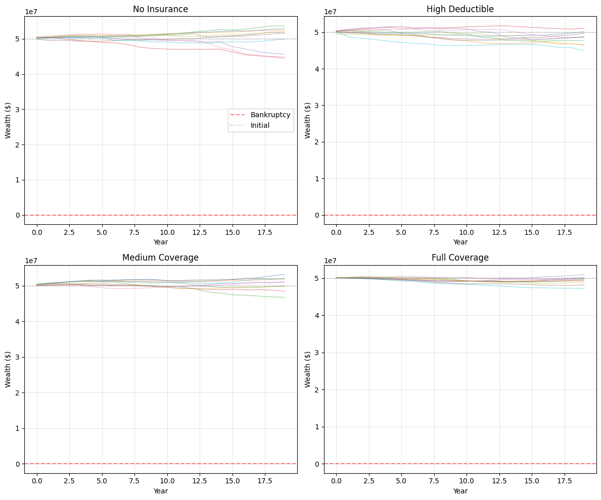
2.5.1. Wealth Trajectories
import matplotlib.pyplot as plt
from ergodic_insurance.simulation import Simulation

# Run simulation with multiple seeds
fig, axes = plt.subplots(2, 2, figsize=(12, 10))
strategies_to_plot = strategies[:4]

for ax, strategy in zip(axes.flat, strategies_to_plot):
    # Run 10 simulations with different seeds for this strategy
    trajectories = []

    for seed in range(10):
        # Create insurance policy for this strategy
        if strategy['limit'] > 0:
            strategy_layer = InsuranceLayer(
                attachment_point=strategy['attachment'],
                limit=strategy['limit'],
                rate=strategy['base_premium_rate']
            )
            strategy_policy = InsurancePolicy(
                layers=[strategy_layer],
                deductible=strategy['attachment']
            )
        else:
            # No insurance case
            strategy_policy = InsurancePolicy(layers=[], deductible=float('inf'))

        # Create and run simulation
        strategy_sim = Simulation(
            manufacturer=heavy_industry.copy(),  # Use a copy for independence
            claim_generator=[standard_losses, catastrophic_risk, operational_risk],
            insurance_policy=strategy_policy,
            time_horizon=20,
            seed=seed
        )

        result = strategy_sim.run()

        # Extract wealth trajectory from the assets array
        trajectories.append(result.assets)

    # Plot trajectories
    for traj in trajectories:
        ax.plot(range(len(traj)), traj, alpha=0.5, linewidth=0.8)

    ax.axhline(y=0, color='red', linestyle='--', alpha=0.5, label='Bankruptcy')
    ax.axhline(y=heavy_industry.config.initial_assets, color='gray',
               linestyle=':', alpha=0.5, label='Initial')
    ax.set_title(strategy['name'])
    ax.set_xlabel('Year')
    ax.set_ylabel('Wealth ($)')
    ax.grid(True, alpha=0.3)

    # Only show legend on first subplot
    if ax == axes.flat[0]:
        ax.legend(loc='best')

plt.tight_layout()
plt.show()
2.5.1.1. Sample Output
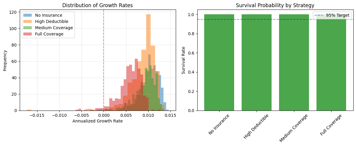
2.5.2. Distribution of Outcomes
# Plot distribution of final wealth
fig, axes = plt.subplots(1, 2, figsize=(12, 5))

# Growth rate distribution
ax1 = axes[0]
for name, results in results_comparison.items():
    ax1.hist(results.growth_rates, bins=30, alpha=0.5, label=name)
ax1.axvline(x=0, color='red', linestyle='--', alpha=0.5)
ax1.set_xlabel('Annualized Growth Rate')
ax1.set_ylabel('Frequency')
ax1.set_title('Distribution of Growth Rates')
ax1.legend()
ax1.grid(True, alpha=0.3)

# Survival analysis
ax2 = axes[1]
names = list(results_comparison.keys())
# Calculate survival rates from ruin_probability
survival_rates = [1 - results_comparison[name].ruin_probability for name in names]
colors = ['red' if sr < 0.95 else 'green' for sr in survival_rates]
ax2.bar(names, survival_rates, color=colors, alpha=0.7)
ax2.axhline(y=0.95, color='blue', linestyle='--', alpha=0.5, label='95% Target')
ax2.set_ylabel('Survival Rate')
ax2.set_title('Survival Probability by Strategy')
ax2.legend()
ax2.set_ylim([0, 1.05])
plt.xticks(rotation=45)

plt.tight_layout()
plt.show()
2.5.2.1. Sample Output
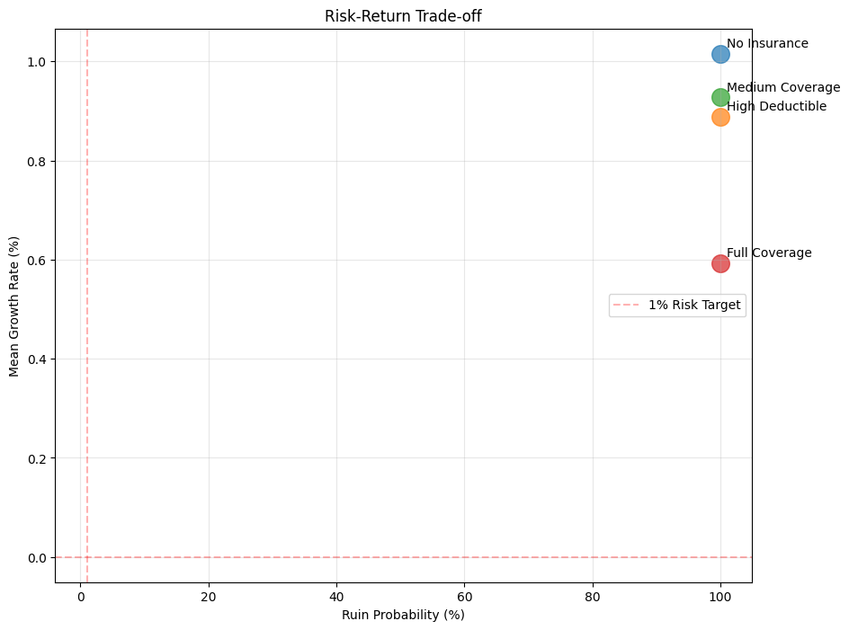
2.5.3. Risk-Return Scatter
# Create risk-return scatter plot
plt.figure(figsize=(10, 8))

for name, results in results_comparison.items():
    mean_return = np.mean(results.growth_rates)
    risk = 1 - results.ruin_probability  # Ruin probability as risk

    plt.scatter(risk * 100, mean_return * 100, s=200, alpha=0.7)
    plt.annotate(name, (risk * 100, mean_return * 100),
                xytext=(5, 5), textcoords='offset points')

plt.xlabel('Ruin Probability (%)')
plt.ylabel('Mean Growth Rate (%)')
plt.title('Risk-Return Trade-off')
plt.grid(True, alpha=0.3)

# Add efficient frontier concept
plt.axhline(y=0, color='red', linestyle='--', alpha=0.3)
plt.axvline(x=1, color='red', linestyle='--', alpha=0.3, label='1% Risk Target')
plt.legend(loc='best')
plt.show()
2.5.3.1. Sample Output
2.6. Advanced Simulation Features
2.6.1. Using Different Random Processes
from ergodic_insurance.stochastic_processes import GeometricBrownianMotion, StochasticConfig
from ergodic_insurance.simulation import Simulation

# Create a stochastic process for revenue volatility
# This adds market volatility to the manufacturer's revenue generation
stochastic_config = StochasticConfig(
    drift=0.05,         # 5% drift (growth trend)
    volatility=0.15,    # 15% volatility (market uncertainty)
    time_step=1.0,      # Annual time step
    random_seed=42      # For reproducibility
)

gbm = GeometricBrownianMotion(stochastic_config)

# Create a stochastic version of heavy_industry
stochastic_manufacturer = WidgetManufacturer(
    config=heavy_industry.config,  # Use same configuration
    stochastic_process=gbm         # Add stochastic process
)

# Compare deterministic vs stochastic simulations
comparison_results = {}

# Run deterministic simulation (no stochastic process)
print("Running deterministic simulation...")
deterministic_sim = Simulation(
    manufacturer=heavy_industry.copy(),
    claim_generator=[standard_losses],
    insurance_policy=insurance_policy,
    time_horizon=20,
    seed=42
)
det_result = deterministic_sim.run()
comparison_results['Deterministic'] = det_result

# Run stochastic simulation (with GBM process)
print("Running stochastic simulation...")
stochastic_sim = Simulation(
    manufacturer=stochastic_manufacturer.copy(),
    claim_generator=[standard_losses],
    insurance_policy=insurance_policy,
    time_horizon=20,
    seed=42
)
# Note: The step() method in manufacturer will apply stochastic shocks when available
stoch_result = stochastic_sim.run()
comparison_results['Stochastic'] = stoch_result

# Compare results
print("\n" + "="*50)
print("Deterministic vs Stochastic Comparison")
print("="*50)

for name, result in comparison_results.items():
    stats = result.summary_stats()
    print(f"\n{name} Simulation:")
    print(f"  Final Assets: ${stats['final_assets']:,.0f}")
    print(f"  Mean ROE: {stats['mean_roe']:.2%}")
    print(f"  ROE Volatility: {stats['roe_std']:.2%}")
    print(f"  Survived: {stats['survived']}")
    if not stats['survived']:
        print(f"  Insolvency Year: {result.insolvency_year}")
2.6.1.1. Sample Output
==================================================
Deterministic vs Stochastic Comparison
==================================================

Deterministic Simulation:
  Final Assets: $51,132,355
  Mean ROE: 1.72%
  ROE Volatility: 0.53%
  Survived: True

Stochastic Simulation:
  Final Assets: $55,664,614
  Mean ROE: 1.95%
  ROE Volatility: 0.64%
  Survived: True
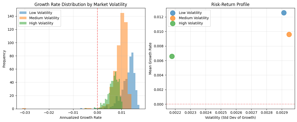
2.6.2. Monte Carlo with Stochastic Processes
This shows how market volatility affects insurance strategy effectiveness
# Create manufacturers with different volatility levels
volatility_scenarios = {
    "Low Volatility": StochasticConfig(drift=0.03, volatility=0.05, random_seed=42),
    "Medium Volatility": StochasticConfig(drift=0.03, volatility=0.15, random_seed=42),
    "High Volatility": StochasticConfig(drift=0.03, volatility=0.25, random_seed=42)
}

# Test with medium coverage insurance strategy
test_insurance = InsuranceProgram(layers=[
    EnhancedInsuranceLayer(
        attachment_point=500_000,
        limit=5_000_000,
        base_premium_rate=0.015
    )
])

# Run Monte Carlo for each volatility scenario
volatility_results = {}

for vol_name, stoch_config in volatility_scenarios.items():
    print(f"Running Monte Carlo for {vol_name}...")

    # Create manufacturer with stochastic process
    gbm_process = GeometricBrownianMotion(stoch_config)
    vol_manufacturer = WidgetManufacturer(
        config=heavy_industry.config,
        stochastic_process=gbm_process
    )

    # Configure Monte Carlo
    mc_config = SimulationConfig(
        n_simulations=500,
        n_years=20,
        parallel=False,
        progress_bar=False,
        seed=42
    )

    # Run Monte Carlo
    mc_engine = MonteCarloEngine(
        loss_generator=mc_loss_generator,
        insurance_program=test_insurance,
        manufacturer=vol_manufacturer,
        config=mc_config
    )

    vol_results = mc_engine.run()
    volatility_results[vol_name] = vol_results

# Analyze impact of volatility
print("\n" + "="*60)
print("Impact of Market Volatility on Insurance Effectiveness")
print("="*60)
print(f"{'Scenario':<20} {'Survival':<12} {'Mean Growth':<15} {'Growth Vol':<12}")
print("-"*60)

for name, results in volatility_results.items():
    survival = 1 - results.ruin_probability
    mean_growth = np.mean(results.growth_rates)
    growth_vol = np.std(results.growth_rates)
    print(f"{name:<20} {survival:>10.1%}   {mean_growth:>12.2%}   {growth_vol:>10.2%}")

# Visualize the results
fig, axes = plt.subplots(1, 2, figsize=(12, 5))

# Growth rate distributions
ax1 = axes[0]
for name, results in volatility_results.items():
    ax1.hist(results.growth_rates, bins=30, alpha=0.5, label=name)
ax1.axvline(x=0, color='red', linestyle='--', alpha=0.5)
ax1.set_xlabel('Annualized Growth Rate')
ax1.set_ylabel('Frequency')
ax1.set_title('Growth Rate Distribution by Market Volatility')
ax1.legend()
ax1.grid(True, alpha=0.3)

# Risk-return scatter
ax2 = axes[1]
for name, results in volatility_results.items():
    mean_return = np.mean(results.growth_rates)
    vol_return = np.std(results.growth_rates)
    survival = 1 - results.ruin_probability
    # Size proportional to survival rate
    ax2.scatter(vol_return, mean_return, s=survival*200, alpha=0.7, label=name)

ax2.set_xlabel('Volatility (Std Dev of Growth)')
ax2.set_ylabel('Mean Growth Rate')
ax2.set_title('Risk-Return Profile')
ax2.legend()
ax2.grid(True, alpha=0.3)

# Add efficient frontier reference line
ax2.axhline(y=0, color='red', linestyle='--', alpha=0.3)

plt.tight_layout()
plt.show()
2.6.2.1. Sample Output
============================================================
Impact of Market Volatility on Insurance Effectiveness
============================================================
Scenario             Survival     Mean Growth     Growth Vol
------------------------------------------------------------
Low Volatility           100.0%          1.26%        0.29%
Medium Volatility        100.0%          0.96%        0.29%
High Volatility          100.0%          0.66%        0.22%
2.6.3. Parallel Processing
# Parallel processing considerations on Windows
# Note: On Windows, parallel processing often has significant overhead due to process spawning
# It's only beneficial for large simulations (typically >5000 simulations)

import time
import warnings

# Create insurance program for test
parallel_insurance = InsuranceProgram(layers=[
    EnhancedInsuranceLayer(
        attachment_point=1_000_000,
        limit=10_000_000,
        base_premium_rate=0.02
    )
])

print("="*60)
print("Parallel Processing Performance Test")
print("="*60)

# Test with different simulation sizes
test_sizes = [500, 1000, 5000, 10000]
results_comparison = {}

for n_sims in test_sizes:
    print(f"\nTesting with {n_sims} simulations:")
    print("-" * 40)

    # Sequential execution
    start_time = time.time()
    sequential_config = SimulationConfig(
        n_simulations=n_sims,
        n_years=20,  # Reduced years for faster testing
        parallel=False,
        progress_bar=False,  # Disable for cleaner output
        seed=42
    )

    sequential_engine = MonteCarloEngine(
        loss_generator=mc_loss_generator,
        insurance_program=parallel_insurance,
        manufacturer=heavy_industry.copy(),
        config=sequential_config
    )

    with warnings.catch_warnings():
        warnings.simplefilter("ignore")
        sequential_results = sequential_engine.run()
    sequential_time = time.time() - start_time

    # Standard parallel execution (not enhanced)
    start_time = time.time()
    parallel_config = SimulationConfig(
        n_simulations=n_sims,
        n_years=20,
        parallel=True,
        n_workers=-2,
        use_enhanced_parallel=False,  # Disable enhanced parallel to avoid Windows issues
        progress_bar=False,
        seed=42
    )

    parallel_engine = MonteCarloEngine(
        loss_generator=mc_loss_generator,
        insurance_program=parallel_insurance,
        manufacturer=heavy_industry.copy(),
        config=parallel_config
    )

    with warnings.catch_warnings():
        warnings.simplefilter("ignore")
        parallel_results = parallel_engine.run()
    parallel_time = time.time() - start_time

    # Store results
    results_comparison[n_sims] = {
        'sequential_time': sequential_time,
        'parallel_time': parallel_time,
        'speedup': sequential_time / parallel_time if parallel_time > 0 else 0
    }

    print(f"  Sequential: {sequential_time:.2f}s")
    print(f"  Parallel:   {parallel_time:.2f}s")
    print(f"  Speedup:    {results_comparison[n_sims]['speedup']:.2f}x")

    # Verify results match
    seq_survival = 1 - sequential_results.ruin_probability
    par_survival = 1 - parallel_results.ruin_probability
    if abs(seq_survival - par_survival) < 0.01:
        print(f"  ✓ Results match (survival ~{seq_survival:.1%})")
    else:
        print(f"  ⚠ Results differ: seq={seq_survival:.1%}, par={par_survival:.1%}")

# Recommendations
print("\n" + "="*60)
print("Recommendations for Your System")
print("="*60)

# Find crossover point
efficient_threshold = None
for n_sims, data in results_comparison.items():
    if data['speedup'] > 1.1:  # 10% improvement threshold
        efficient_threshold = n_sims
        break

if efficient_threshold:
    print(f"✓ Use parallel execution for simulations > {efficient_threshold}")
    print(f"  (Achieves {results_comparison[efficient_threshold]['speedup']:.1f}x speedup)")
else:
    print("⚠ On this system, sequential execution is generally faster")
    print("  due to parallel processing overhead.")
    print("\nFor better parallel performance:")
    print("  - Use larger simulation counts (>5000)")
    print("  - Use Linux/Mac where process spawning is faster")
    print("  - Consider using enhanced parallel with shared memory (if available)")
2.6.3.1. Sample Output
============================================================
Parallel Processing Performance Test
============================================================

Testing with 500 simulations:
----------------------------------------
  Sequential: 1.13s
  Parallel:   1.00s
  Speedup:    1.13x
  ✓ Results match (survival ~100.0%)

Testing with 1000 simulations:
----------------------------------------
  Sequential: 2.07s
  Parallel:   1.89s
  Speedup:    1.10x
  ✓ Results match (survival ~100.0%)

Testing with 5000 simulations:
----------------------------------------
  Sequential: 8.74s
  Parallel:   8.72s
  Speedup:    1.00x
  ✓ Results match (survival ~100.0%)

Testing with 10000 simulations:
----------------------------------------
  Sequential: 17.61s
  Parallel:   16.77s
  Speedup:    1.05x
  ✓ Results match (survival ~100.0%)
2.7. Best Practices
2.7.1. 1. Choose Appropriate Time Horizons
Short-term (1-5 years): Focus on survival
Medium-term (5-20 years): Balance growth and safety
Long-term (20+ years): Ergodic effects dominate
2.7.2. 2. Set Realistic Parameters
2.7.3. 3. Validate Results
# Sanity checks for simulation results
def validate_simulation(result, manufacturer):
    """Validate simulation results for reasonableness."""

    # Calculate growth rate from assets
    if len(result.assets) > 1:
        initial_assets = result.assets[0]
        final_assets = result.assets[-1]
        n_years = len(result.assets) - 1
        if initial_assets > 0 and final_assets > 0:
            annualized_growth = (final_assets / initial_assets) ** (1/n_years) - 1
        else:
            annualized_growth = -1.0
    else:
        annualized_growth = 0.0

    # Get stats for validation
    stats = result.summary_stats()

    checks = {
        "Positive initial wealth": result.assets[0] > 0,
        "Reasonable growth": -0.5 < annualized_growth < 0.5,
        "Trajectory length matches years": len(result.assets) == len(result.years),
        "Final wealth matches stats": abs(stats['final_assets'] - result.assets[-1]) < 1,
        "ROE array length matches": len(result.roe) == len(result.years),
        "No NaN in assets": not np.any(np.isnan(result.assets)),
        "Survived matches insolvency": (result.insolvency_year is None) == stats['survived']
    }

    print("Simulation Validation Results:")
    print("-" * 40)
    for check, passed in checks.items():
        status = "✅" if passed else "❌"
        print(f"{status} {check}")

    # Additional info
    print("\nKey Metrics:")
    print(f"  Initial Assets: ${result.assets[0]:,.0f}")
    print(f"  Final Assets: ${result.assets[-1]:,.0f}")
    print(f"  Annualized Growth: {annualized_growth:.2%}")
    print(f"  Mean ROE: {stats['mean_roe']:.2%}")
    print(f"  Simulation Years: {len(result.years)}")
    print(f"  Survived: {stats['survived']}")

    return all(checks.values())

# Validate the deterministic simulation result
is_valid = validate_simulation(det_result, heavy_industry)
print(f"\n{'✅ Simulation is valid!' if is_valid else '❌ Simulation has issues!'}")
2.7.3.1. Sample Output
Simulation Validation Results:
----------------------------------------
✅ Positive initial wealth
✅ Reasonable growth
✅ Trajectory length matches years
✅ Final wealth matches stats
✅ ROE array length matches
✅ No NaN in assets
✅ Survived matches insolvency

Key Metrics:
  Initial Assets: $50,187,227
  Final Assets: $51,132,355
  Annualized Growth: 0.10%
  Mean ROE: 1.72%
  Simulation Years: 20
  Survived: True

✅ Simulation is valid!
2.8. Troubleshooting Common Issues
2.8.1. Issue: Simulation runs too slowly
Solution: Reduce number of simulations or use parallel processing.
2.8.2. Issue: All paths show bankruptcy
Solution: Check if losses are too severe relative to assets.
2.8.3. Issue: Results vary wildly between runs
Solution: Increase simulation count and use seeds for diagnostic stability.
2.9. Next Steps
Now that you understand basic simulations:
Configuring Insurance: Learn about multi-layer programs
Optimization Workflow: Find optimal insurance parameters
Analyzing Results: Deep dive into metrics and decisions
2.10. Summary
You’ve learned how to:
✅ Configure manufacturer models for different industries
✅ Generate various loss distributions
✅ Run single-path and Monte Carlo simulations
✅ Compare insurance strategies
✅ Visualize and interpret results
✅ Apply best practices and troubleshoot issues
You’re now ready to explore more complex insurance structures and optimization!