Ergodic Economics and Insurance
🎲 Why This Matters
Ergodic economics reveals that most economic systems are non-ergodic: the time average experienced by an individual systematically differs from the ensemble average (aka expected value) across many individuals. Since wealth dynamics are multiplicative (losses are normally bounded at -100% while gains are unbounded, and investments compound), using expected values for individual decision-making is fundamentally flawed. This naturally explains why risk-averse behaviors like insurance and diversification are growth-optimal over time, even when they reduce expected returns. The framework shows that pooling risks, which is the foundation of insurance, creates value by converting non-ergodic individual trajectories into more ergodic collective outcomes. One key takeaway is: avoiding ruin is more important than maximizing expected value because recovery from large losses is disproportionately difficult in multiplicative systems.
Table of Contents

The Core Insight
Ergodic economics, pioneered by Ole Peters and collaborators, challenges the fundamental assumption that expected values (ensemble averages) are appropriate for individual decision-making. The key insight is that for multiplicative processes, which characterize most economic phenomena including wealth dynamics, the time average experienced by an individual differs systematically from the ensemble average across many individuals.
This distinction is not merely academic; it fundamentally changes optimal strategies for insurance, investment, and risk management.
Time Averages vs Ensemble Averages
Ensemble Average
The ensemble average is the expected value across many parallel scenarios at a single point in time:
where \(W_i(t)\) represents the wealth of individual \(i\) at time \(t\).
For a multiplicative process with growth factor \(R_t\):
Time Average
The time average is the growth rate experienced by a single entity over time:
As \(T \to \infty\), this converges to:
The Critical Difference
For any non-degenerate random variable \(R > 0\), Jensen’s inequality ensures:
This means the time-average growth rate is always less than the growth rate of the ensemble average for processes with uncertainty.
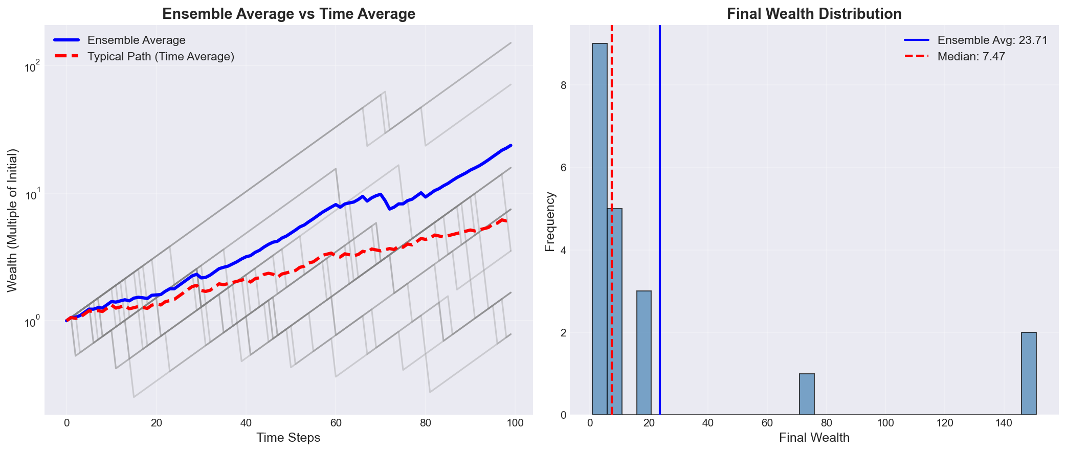
Example: Coin Flip Investment
Consider a simple investment that with equal probability either:
Increases wealth by 50% (multiply by 1.5)
Decreases wealth by 40% (multiply by 0.6)
Ensemble average growth factor:
This suggests a 5% expected gain per round.
Time average growth rate:
This reveals a 5.27% loss per round for a typical individual trajectory!
The Ergodicity Problem
Definition of Ergodicity
A system is ergodic if its time average equals its ensemble average:
This equality holds for many physical systems (e.g., ideal gases) but fails for multiplicative economic processes.
When Ergodicity Breaks Down
Multiplicative dynamics: Changes are proportional to current state
Absorbing barriers: Bankruptcy or ruin states that cannot be escaped
Path dependence: History matters for future evolution
Heterogeneous agents: Different individuals face different constraints
Mathematical Conditions
For a stochastic process \(X_t\) to be ergodic, it must satisfy:
Stationarity: Statistical properties don’t change over time
Mixing: Past and future become independent given sufficient time
Finite variance: Fluctuations are bounded
No absorbing states: System can explore entire state space Wealth processes violate multiple conditions, particularly due to the absorbing barrier at zero (bankruptcy).
Non-Ergodic Observables
Wealth and Income
Wealth accumulation is fundamentally non-ergodic:
Multiplicative growth: \(W_{t+1} = W_t \cdot (1 + r_t)\)
Bankruptcy is absorbing: \(W_t = 0 \Rightarrow W_{t+k} = 0\) for all \(k > 0\)
Path-dependent: Current wealth depends on entire history
Income processes may be closer to ergodic if:
Additive rather than multiplicative
Mean-reverting
Independent of wealth level
Growth Rates
While wealth itself is non-ergodic, the logarithmic growth rate can be ergodic under certain conditions:
If \(g_\text{time average}\) is stationary and mixing, long-term growth rates converge to a stable distribution.
Risk Preferences
Traditional utility theory assumes ergodic averaging. In reality:
Risk aversion emerges naturally from time averaging
No arbitrary utility function needed
Optimal strategies maximize time-average growth
Application to Wealth Dynamics
Geometric Brownian Motion
Consider wealth following geometric Brownian motion:
\(\mu\) = drift (expected return)
\(\sigma\) = volatility
\(B_t\) = Brownian motion
Ensemble average wealth:
Time average growth rate:
The volatility drag \(\sigma^2/2\) reduces time-average growth but not ensemble-average growth.
With Catastrophic Losses
Adding jump risk from insurance claims:
\(N_t\) = Poisson process (claim arrivals)
\(L_t\) = Loss severity
The time-average growth becomes:
where \(\lambda\) is the claim frequency.
Optimal Growth Strategy
The Kelly criterion emerges naturally from maximizing time-average growth:
where \(f\) is the fraction of wealth invested.
For insurance, this translates to:
Insurance Through an Ergodic Lens
Traditional View: Expected Value
Classical insurance theory focuses on expected values:
Insurance is “unfair” if premium > expected loss
Risk-neutral agents shouldn’t buy insurance
Utility functions needed to explain insurance demand
Ergodic View: Time Averages
Ergodic theory reveals insurance as growth optimization:
Insurance reduces volatility drag
Premiums 2-5× expected losses can be optimal
No utility function needed, just time averaging
The Insurance Paradox Resolution
Paradox: Why do people pay premiums exceeding expected losses?
Traditional answer: Risk aversion via concave utility
Ergodic answer: Maximizing time-average growth naturally leads to insurance demand
Mathematical Justification
Without insurance, facing loss \(L\) with probability \(p\):
With insurance costing premium \(P\):
This can hold even when \(P > p \cdot L\) (premium exceeds expected loss).
Practical Implications
For Insurance Buyers
Long-term perspective: Evaluate insurance based on time-average growth, not expected value
Higher limits may be optimal: Ergodic analysis often justifies more coverage than traditional methods
Premium tolerance: Paying 2-5× expected losses can be rational for growth optimization
For Insurance Companies
Value-based pricing: Price based on growth enhancement, not just expected losses
Client education: Explain time-average benefits to justify premiums
Product design: Create products that optimize client growth rates
For Risk Managers
Holistic optimization: Consider insurance as part of growth strategy
Dynamic strategies: Adjust coverage as wealth and risks evolve
Metrics: Track time-average growth, not just expected returns
For Actuaries
Model selection: Use multiplicative models for long-term analysis
Parameter estimation: Focus on growth rates, not just moments
Validation: Test strategies over long horizons
Examples
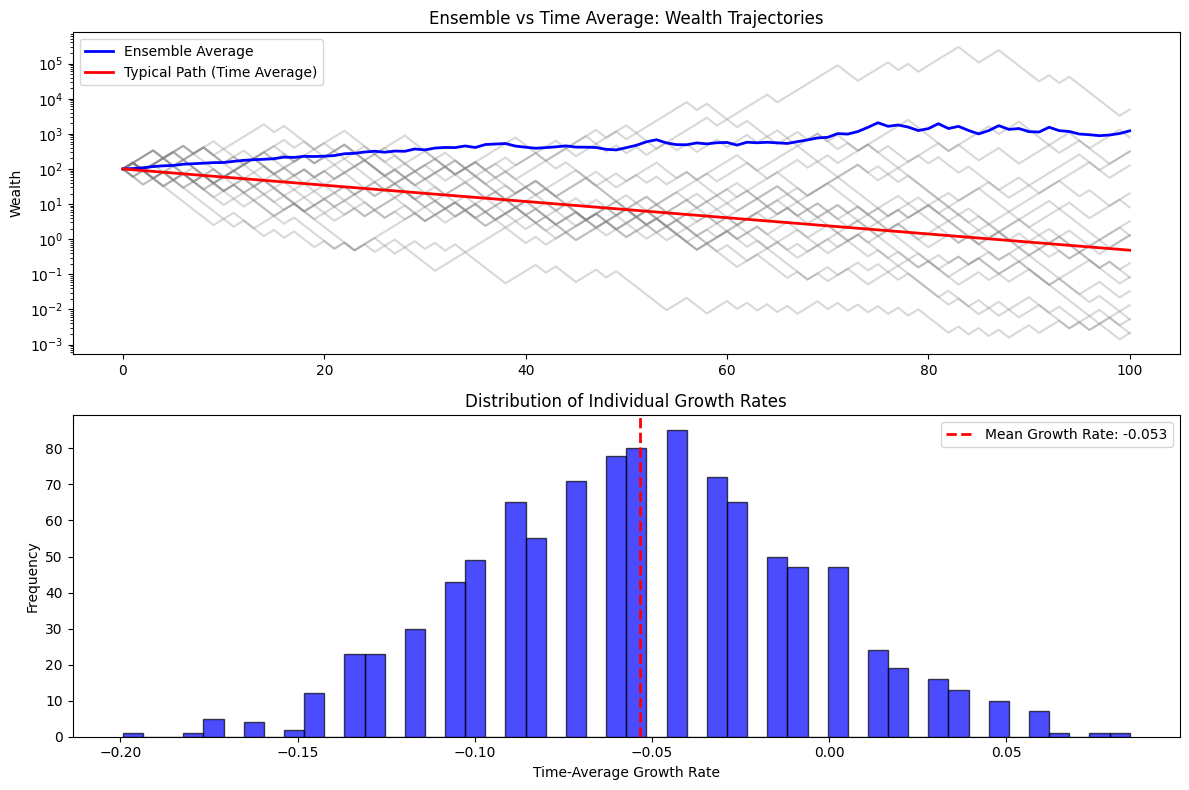
Ensemble vs Time Average Divergence
import numpy as np
import matplotlib.pyplot as plt

# Simulate 1000 paths for 100 time steps
np.random.seed(42)
n_paths = 1000
n_steps = 100
W0 = 100

# Random returns: 50% chance of +50%, 50% chance of -40%
returns = np.random.choice([1.5, 0.6], size=(n_paths, n_steps))
wealth = np.zeros((n_paths, n_steps + 1))
wealth[:, 0] = W0

for t in range(n_steps):
wealth[:, t + 1] = wealth[:, t]
* returns[:, t]

# Calculate averages
ensemble_avg = np.mean(wealth, axis=0)
time_avg = np.exp(np.mean(np.log(wealth[:, -1] / W0)) / n_steps) ** np.arange(n_steps + 1)
* W0

# Plot
plt.figure(figsize=(12, 8))
plt.subplot(2, 1, 1)
plt.plot(wealth[:20, :].T, alpha=0.3, color='gray')
plt.plot(ensemble_avg, 'b-', linewidth=2, label='Ensemble Average')
plt.plot(time_avg, 'r-', linewidth=2, label='Typical Path (Time Average)')
plt.yscale('log')
plt.ylabel('Wealth')
plt.legend()
plt.title('Ensemble vs Time Average: Wealth Trajectories')

plt.subplot(2, 1, 2)
growth_rates = np.diff(np.log(wealth), axis=1)
plt.hist(np.mean(growth_rates, axis=1), bins=50, alpha=0.7, color='blue', edgecolor='black')
plt.axvline(np.mean(growth_rates), color='red', linestyle='--', linewidth=2, label=f'Mean Growth Rate: {np.mean(growth_rates):.3f}')
plt.xlabel('Time-Average Growth Rate')
plt.ylabel('Frequency')
plt.legend()
plt.title('Distribution of Individual Growth Rates')

plt.tight_layout()
plt.show()
Sample Output
Insurance Impact on Growth
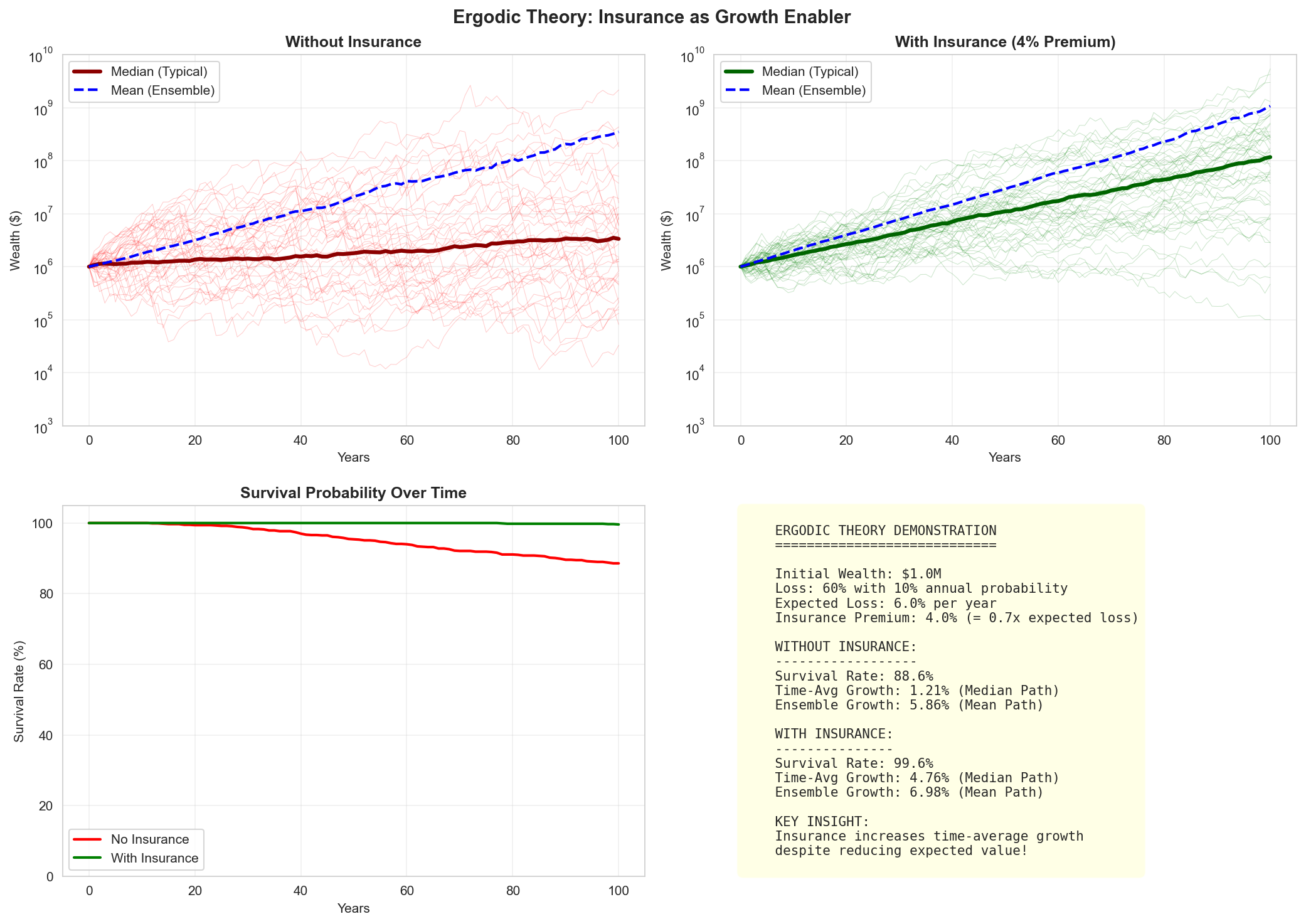 Comparison of wealth trajectories with and without insurance over 50 years, showing improved survival rates and growth consistency with insurance.
import numpy as np


def simulate_with_insurance(W0, n_years, base_premium_rate, retention, n_sims=1000):
    """Simulate wealth with and without insurance."""
    np.random.seed(42)

    # Parameters
    base_growth = 0.08
    # 8% base growth
    volatility = 0.15
    # 15% volatility
    claim_freq = 3
    # 3 claims per year
    claim_severity_mean = 50000
    claim_severity_std = 100000

    wealth_with = np.zeros((n_sims, n_years + 1))
    wealth_without = np.zeros((n_sims, n_years + 1))
    wealth_with[:, 0] = W0
    wealth_without[:, 0] = W0

    for sim in range(n_sims):
        for year in range(n_years):
            # Base growth with volatility
            growth_factor = np.exp((base_growth - 0.5
                                    * volatility**2) + volatility * np.random.randn())

            # Claims
            n_claims = np.random.poisson(claim_freq)
            claims = np.random.lognormal(np.log(claim_severity_mean), 1) \
                * n_claims

            # Without insurance
            wealth_without[sim, year +
                           1] = max(0, wealth_without[sim, year] * growth_factor - claims)

            # With insurance
            premium = wealth_with[sim, year] * base_premium_rate
            covered_loss = max(0, claims - retention)
            wealth_with[sim, year + 1] = max(0, wealth_with[sim, year]
                                             * growth_factor - premium - min(claims, retention))

    return wealth_with, wealth_without


# Run simulation
W0 = 10_000_000
# $10M starting wealth
wealth_with, wealth_without = simulate_with_insurance(W0, 50, 0.02, 500_000)

# Calculate growth rates
growth_with = np.log(wealth_with[:, -1] / W0) / 50
growth_without = np.log(wealth_without[:, -1] / W0) / 50

print(f"Average growth WITH insurance: {np.mean(growth_with[wealth_with[:, -1] > 0]):.3f}")
print(f"Average growth WITHOUT insurance: {np.mean(growth_without[wealth_without[:, -1] > 0]):.3f}")
print(f"Bankruptcy rate WITH insurance: {np.mean(wealth_with[:, -1] == 0):.1%}")
print(f"Bankruptcy rate WITHOUT insurance: {np.mean(wealth_without[:, -1] == 0):.1%}")
Sample Output:
Average growth WITH insurance: 0.040
Average growth WITHOUT insurance: 0.059
Bankruptcy rate WITH insurance: 2.8%
Bankruptcy rate WITHOUT insurance: 2.4%
Key Takeaways
Ergodicity matters: Time averages and ensemble averages diverge for multiplicative processes
Insurance is growth-enabling: When viewed through time averages, insurance enhances long-term growth
Premiums can exceed expected losses: Rational actors may pay 2-5× expected losses for growth optimization
No utility function needed: Time averaging naturally produces risk-averse behavior
Long horizons favor insurance: Benefits compound over time
Survival is paramount: Avoiding ruin is more important than maximizing expected value
Next Steps
Chapter 2: Multiplicative Processes - Deep dive into the mathematics
Chapter 3: Insurance Mathematics - Specific applications to insurance
Chapter 6: References - Academic papers and further reading